DOCK 6.13 Users Manual
Principal contributors to the current code:
William Joseph Allen (TACC)
Trent Balius (FNLCR)
John Bickel (SUNY-Stony Brook)
Brock Boysan (SUNY-Stony Brook)
Scott R. Brozell (Rutgers University)
Chris Corbo (SUNY-Stony Brook)
Brian Fochtman (SUNY-Stony Brook)
Lingling Jiang (Columbia University)
P. Therese Lang (UCB)
Guilherme D. R. Matos (SUNY-Stony Brook)
T. Dwight McGee Jr. (SUNY-Stony Brook)
Demetri Moustakas (Harvard)
Sudipto Mukherjee (Temple)
Owen O'Reilly (SUNY-Stony Brook
Steven Pak (SUNY-Stony Brook)
Lauren Prentis (SUNY-Stony Brook)
Courtney Singleton (SUNY-Stony Brook)
Yuchen Zhou (SUNY-Stony Brook)
Robert Rizzo (SUNY-Stony Brook)
David Case (Rutgers University)
Brian Shoichet (UCSF)
Irwin Kuntz (UCSF)
For more information about previous contributors, please see the History .
Copyright © 2006-2025
Regents of the University of California
All Rights Reserved
Last updated June 8, 2025
1.3. Installation
1.4. What's New in DOCK 6
1.5. Overview of
the DOCK Suite of Programs
2.
DOCK
2.1.
Overview
2.2.
History
2.3.
Command-line Arguments
2.4.
The Parameter Parser
2.5.
Sampling Methods
2.5.1.
Rigid and Flexible Ligand Docking
2.5.1.1
Anchor and Grow
2.5.1.2
Identification of Rigid Segments
2.5.1.3
Manual Specifications of Non-Rotatable Bonds
2.5.1.4
Pruning the Conformation Search Tree
2.5.1.5
Time Requirements
2.5.1.6
Growth Tree and Statistics
2.5.1.7
Rigid Body and Flexible Ligand Docking Input Parameters
2.5.2.
De novo Design
2.5.2.1.
DOCK_DN Input Parameters
2.5.2.2.
DOCK_D3N Input Parameters
2.5.3.
DOCK_GA: Molecular Evolution using a Genetic Algorithm
2.5.3.1
DOCK_GA Input Parameters
2.5.3.2
DOCK_GA RDKit Input Parameters
2.5.4. Hierarchical DataBase (HDB) Search
2.5.4.1
HDB Input Parameters
2.5.5. Covalent Attach-and-Grow
2.5.5.1
Covalent Input Parameters
2.6.
Fragment Library Generation
2.6.1
Input Parameters
2.7.
Database Filter
2.7.1
Input Parameters
2.7.2 RDKit
Input Parameters
2.8.
Ligand RMSD
2.8.1
Input Parameters
2.9.
Orienting the Ligand
2.9.1.
Sphere Matching
2.9.2.
Critical Points
2.9.3.
Chemical Matching
2.9.4.
Macromolecular Docking
2.9.5.
Input Parameters
2.10. Internal Energy Calculation
2.10.5.
Input Parameters
2.11. Scoring
2.11.1. Bump Filter
2.11.2. Contact Score
2.11.3. Grid-Based Score
2.11.4. DOCK 3.5 Score
2.11.5. Continuous Score
2.11.6. Zou GB/SA Score
2.11.7. Hawkins GB/SA Score
2.11.8. AMBER Score
2.11.8.1. AMBER Score Binding Energy
2.11.8.2. AMBER Score Receptor Flexibility
2.11.8.3. AMBER Score Inputs
2.11.8.4. AMBER Score Outputs
2.11.8.5. AMBER Score in Practice
2.11.8.6. AMBER Score Parameters
2.11.9. Footprint Score
2.11.10. MultiGrid FPS Score
2.11.11. Pharmacophore Matching Similarity Score
2.11.12. Internal Energy Score
2.11.13. SASA Score
2.11.14. GIST Score
2.11.15. Descriptor Score
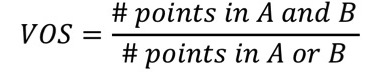
2.11.15.1. Tanimoto Score
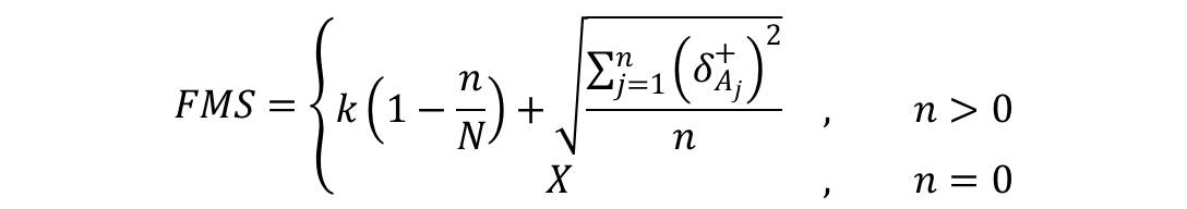
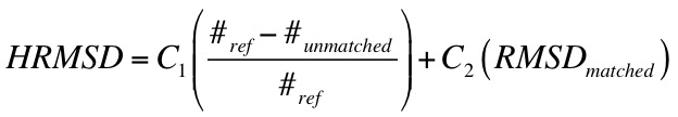
2.11.15.2. Hungarian Matching Similarity Score
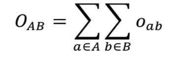
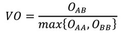
2.11.15.3. Volume Overlap Score
2.12. Minimization
2.13.
Miscellaneous Parameters
2.14.
Parameter Files
2.14.1.
Atom Definition Rules
2.14.2.
vdw.defn
2.14.3.
chem.defn
2.14.4.
chem_match.tbl
2.14.5.
ph4.defn
2.14.6.
flex.defn
2.14.7.
flex_drive.tbl
2.15.
Parallel Processing
3.
Accessories
3.1. Grid
3.1.1.
Overview
3.1.2.
Bump Checking
3.1.3.
Contact Scoring
3.1.4.
Energy Scoring
3.2.
Docktools
3.2.1. Chemgrid
3.2.2. Ligand
Desolvation
3.2.3.
Occupancy Desolvation
3.2.4. Grid
Conversion
3.3.
Nchemgrids
3.4.
Sphgen
3.4.1.
Overview
3.4.2.
Critical Points
3.4.3.
Chemical Matching
3.4.4.
Output
3.5.
Showbox
3.6.
Showsphere
3.7.
Sphere Selector
3.8. Antechamber
3.9. tLEaP
3.10.
Amber Score Preparation Scripts
4.
Molecular File Formats
4.1.
Tripos MOL2 Format
4.2.
PDB Format
4.3.
BILD Format
5.
References
6.
Acknowledgments
Introduction
RETURN TO TABLE OF CONTENTS
1.1. General
Overview
DOCK is molecular modeling program used to identify potential binding geometries
and interactions of a molecule to a target. Specifically, docking is the identification of the
low-energy binding modes of a small molecule, or ligand, within the active site of a macromolecule, or
receptor, whose structure is known. A compound that interacts strongly with, or binds,
a receptor associated with a disease may inhibit its function and thus
act as a drug. Solving the docking problem computationally requires an
accurate representation of the molecular energetics as well as an
efficient algorithm to search the potential binding modes.
Historically, the
DOCK algorithm
addressed rigid body docking using a geometric matching algorithm to
superimpose the ligand onto a negative image of the binding pocket.
Important features that improved the algorithm's ability to find the
lowest-energy binding mode, including force-field based scoring,
on-the-fly optimization, an improved matching algorithm for rigid body
docking and an algorithm for flexible ligand docking, have been added
over the years. For more information on past versions of DOCK,
click here.
With the release
of DOCK 6, we continue to improve the algorithm's ability to predict ligand
binding poses by adding new features like
force-field scoring, enhanced solvation models, reference-based scoring options,
and de novo design. For more
information about the current release of DOCK, click here.
RETURN TO TABLE OF CONTENTS
1.2.
What Can DOCK Do for You
We and others have used DOCK for the
following applications:
- predict binding modes of small
molecule-protein complexes
- search databases of ligands for
compounds that mimic the inhibitory binding interactions of an experimentally
validated inhibitor
- search databases of ligands for
compounds that bind a particular site of a specific protein
- search databases of ligands for
compounds that bind nucleic acid targets
- examine possible binding
orientations of protein-protein and protein-DNA complexes
- help guide synthetic efforts by
examining small molecules that are computationally derived
- many more...
RETURN TO TABLE OF CONTENTS
1.3. Installation
DOCK is Unix
based scientific software and
follows a common installation recipe:
download, unpack, configure, build, and test.
The simple configuration scheme of DOCK is based on plain text files.
Building and testing employ the
make
command.
DOCK installation is so simple and transparent that users
have a reasonable chance of correcting problems themselves.
Start with a plain serial installation.
Follow the detailed steps (0. through 5.) enumerated below.
The appropriate configuration option is likely gnu; see step 3.
Subsequently, additional executables can be installed for parallel; see step 6.
(Here is a quick start for an example gnu serial and parallel installation:
cd install; ./configure gnu; make install;
make dockclean; ./configure gnu parallel;
setenv MPI_HOME /bla; make dock; make test;).
If problems occur then read the diagnostics carefully and apply the
scientific method.
Most initial installation problems are due to unavailable or fouled tools,
especially compilers; verify that your compilers work before installing DOCK.
To observe what's under the hood, view the DOCK configuration file
(install/config.h) that is created by configure, especially its troubleshooting
section that describes corrective measures for common difficulties.
Execute make -n for a dry run. Platform idiosyncrasies
can and should be corrected by editing the install/config.h, as opposed to
editing the original source file, e.g., install/gnu.
Consult the FAQ.
Search the
DOCK-Fans mailing list archive.
General use of DOCK does not require setting environment variables.
However, we recommend the name DOCK_HOME for referencing DOCK6. During
installation, paths to some critical locations are hard coded. In
version 6.12, some auxiliary scripts were added in directory
template_pipeline that do employ DOCK_HOME.
NOTE FOR WINDOWS
USERS: DOCK and its accessories must be run using a Unix-like
environment such as Cygwin
( http://www.cygwin.com/ ).
We recommend a full Unix installation.
In particular, when you install your emulator,
make sure to also install compilers, Unix shells, and perl ( Devel for Cygwin ).
All steps below should be performed
using Cygwin or another Unix emulator for Windows.
See also the
DOCK wiki entry for Cygwin.
(0) Check for Bugfixes online.
(1) Unpack the distribution using the following command:
[user@dock ~]
tar -zxvf dock.6.10.tar.gz
(2) Enter the installation directory:
[user@dock ~] cd dock6/install
(3) Configure the Makefile for the
appropriate operating system:
[user@dock ~] ./configure
[configuration file]
AUTHOR: Scott Brozell
USAGE: configure [-help]
[configuration file]
OPTIONS: Notable ones are listed below;
for a complete list see the configure -help output.
-help #emit the usage statement
configuration file #input file
containing operating system appropriate variables
| Configuration Files |
Target |
| gnu |
GNU compilers |
| gnu.acml |
recent GNU compilers and
ACML |
| gnu.parallel |
GNU compilers with parallel processing capability |
| gnu.parallel.rdkit |
GNU compilers with parallel processing capability and
RDKit capability |
| gnu.rdkit |
GNU compilers with RDKit
capability |
| homebrew |
GNU compilers installed on macOS using the Homebrew package manager |
| homebrew.rdkit |
GNU compilers installed on macOS using the Homebrew package manager
with RDKit capability |
| ibmaix |
IBM AIX and native compilers |
| intel |
Intel compilers |
| intel.mkl |
Intel compilers and
MKL |
| intel.parallel |
Intel compilers with parallel processing capability |
| intel.intelmpi.parallel |
Intel compilers with parallel processing capability (specific to Intel MPI) |
| pgi |
PGI compilers |
| sgi |
SGI native compilers |
DESCRIPTION:
Create the DOCK configuration file, config.h, by copying an existing
configuration file that is selected using the arguments. When invoked
without arguments, print this usage statement and if the configuration
file exists then print its creation stamp. Some configuration files
require that environment variables be defined; these requirements are
listed in the files and emitted by configure.
Note that as of version 6.6 gfortran is the default Fortran compiler in
the gnu config files (replacing g77).
In the unlikely case that another Fortran compiler is desired,
simply hand edit install/config.h to use the alternative.
(4) Build the DOCK executables via the following command:
[user@dock ~] make all # builds all
the DOCK programs
Finer control over which executables are built is
available, but is rarely necessary, via one of the following commands:
[user@dock ~] make dock # builds only the dock program
[user@dock ~] make utils # builds only the accessory programs
(5)
Test the built executables via this command:
[user@dock ~] make test
The test directory contains the DOCK quality control
(QC) suite. It produces pass/fail results via fast regression tests.
The suite should complete in less than ten minutes; five minutes is typical.
Un-passed tests should be examined to determine their significance.
The make test command from the install directory is a shortcut for this
sequence: cd test; make test; make check.
The make check command executed from the test directory emits all
the differences uncovered during testing.
The make clean command executed from the test directory removes all files
produced during testing; this command is automatically
executed by the main make test command above; however, to run tests from
a subdirectory of the test directory, one should explicitly execute make clean.
NOTE: Some failures are not significant.
For example, differences in the tails of floating point numbers may not
be significant. The sources of such differences are frequently
platform dependencies from computer hardware, operating systems,
and compilers that impact arithmetic precision and
random number generators.
In addition, the reference outputs as of version 6.4 are from a 64 bit
platform and as of version 6.10 use gfortran gcc version 7.5.0,
and this can cause false positives on 32 bit platforms or with other compilers;
in particular, differing numbers of Orientations or
Conformations and different Contact or Grid scores.
We are working on increasing the QC suite's resilience to these issues.
For now, apply common sense and good judgment to determine
the significance of a possible failure.
Note that some number of failures is
rarely an indication of real problems, but if almost
every test fails then something is amiss.
Some features of DOCK
(DOCK3.5 Score aka ChemGrid Score)
require an electrostatic potential map which is usually generated by DelPhi.
Testing of these features requires that the environment variable
DELPHI_PATH be defined to the full path of the DelPhi executable.
DelPhi
is not distributed with DOCK; see also
Wikipedia.
Qnifft may now be used to calculate the electrostatic potential map (as is done with DOCK 3.7 and 3.8), instead of Delphi.
Testing of these features with Qnifft requires that the environment variable QNIFFT_PATH be defined (and not DELPHI_PATH) to the full path of the Qnifft executable (this executable is available with DOCK 3.7).
DOCK with
parallel processing capability
will be automatically tested by the QC suite if dock6.mpi has been built.
The same environment variable, MPI_HOME, needed for compilation should
be identically defined for testing.
Optionally, the environment variable DOCK_PROCESSES can be set to
control how many MPI processes are tested.
See step 6 below
for details on building dock6.mpi.
(6) OPTIONAL: Additional dock executables.
(i) DOCK with parallel processing capability
requires a Message Passing Interface (MPI) library.
Because of the vagaries of MPI libraries, building parallel DOCK
has more pitfalls than installing the serial version.
The MPI library must be installed and running on the system if the
parallel features of DOCK are to be used.
The DOCK installation mechanism supports all MPI implementations.
The focus on MPICH2 and MPICH was eliminated in version 6.10.
Once MPI is installed, define the environment variable MPI_HOME
to the top level of the MPI directory.
MPI_HOME will be referenced by all stages of the build procedure -
from configuration through testing.
See the
Parallel DOCK section
for execution information.
NOTE: The parallel configuration files should support
any MPI installation even though they were initially tailored to MPICH.
Linking problems, such as undefined references and cannot find libbla_bla,
can occur due to idiosyncrasies in the MPI installation.
One corrective approach is to use manual linking;
edit your config.h to add to the LIBS definition
the link flags (-L and -l) from the command:
$MPI_HOME/mpicc -show;
in general, the LIBS should contain those link flags in the same order.
(ii) As of version 6.11, DOCK can be compiled with
RDKit.
However, RDKit is not packaged with DOCK. It must be downloaded
and built separately to eventually be compiled with DOCK.
Importantly, for consistency with published work on DOCK6 Using RDKit,
Matos et al. J. Chem. Inf. Model. 2023,
we recommend installing RDKit Release 2019.09.1 which depends on
Boost 1.71.0 and Eigen 3.3.9. If you already have this RDKit installed then
you can build a DOCK executable with support for RDKit by first defining these
environment variables (using Bourne shell syntax):
export BOOST="/path/to/boost/root/dir/"
export RDBASE="/path/to/rdkit/root/dir"
export LD_LIBRARY_PATH="${BOOST}/lib:${RDBASE}/lib:${LD_LIBRARY_PATH}"
and then running the following commands for a serial executable (or their
equivalent for a parallel executable):
cd install; make distclean; ./configure gnu.rdkit;
make dock; make test;.
If you don't have RDKit installed then there are several approaches:
The simplest may be to use the automated recipe supplied by DOCK; see below.
The other approach is to manually install RDKit yourself. This path has several
options; for instructions please refer to this
RDKit website,
and consult the
How is RDKit installed ?
DOCK FAQ for a Python-less approach.
The DOCK automated recipe for installing RDKit requires that you have
anaconda/miniconda installed. After the installation of anaconda/miniconda,
you must export the root path of anaconda/miniconda as "CONDABASE" in your
.bashrc or equivalent file, e.g.:
export CONDABASE="/path/to/miniconda3"
Then you can invoke DOCK's recipe for installing RDKit as shown below:
[user@dock ~] cd ./install
[user@dock ~] make rdkit # downloads RDKit and its dependencies, then compiles. Please follow the instructions shown in the screen.
If you need to clean out the RDKit compiled contents, please
execute the command below. Once you execute that command then
you will not be able to compile DOCK with RDKit unless you rebuild RDKit:
[user@dock ~] make rdkitclean # to clean out everything pertaining to RDKit.
(7) Build the DOCK executables via Docker
In the 6.12 DOCK6 release, DOCK6 can now be compiled in Docker images
(no relation to DOCK6). To start, you must have the
Docker engine installed your local computer. The Docker engine is necessary
to generate the images from Docker files, then to run to DOCK6 program and tools
in a Docker container.
Instructions on how to Dockerize
cd in install/docker./dockerize Dockerfile.gnu_w_parallel. This will start dockerizing the dock6 build. -
Then the
dock6-suite.docker "binary" will be generated in the bin folder.
Please be patient, this will take awhile.
Example Usage
Non-interactive mode:
dock6-suite.docker -b "dock6 -i dn.in -o dn.out"
dock6-suite.docker -b "grid -i grid.in -o grid.out"
dock6-suite.docker -b "dock6 -i dn.in -o dn.out" -v /PATH/TO/FILE1 -v ../../PATH/TO/FILE2 -v /PATH/TO/DIR
dock6-suite.docker -b "mpirun -n 4 dock6.mpi -i dn.in -o dn.out"
Interactive mode:
dock6-suite.docker
dock6-suite.docker -v /PATH/TO/FILE1 -v ../../PATH/TO/FILE2 -v /PATH/TO/DIR
Usage flags
Usage: dock6-suite.docker [ -h help ] [ -b BINARY CALL WITH ARGUMENTS ] [ -v mounting files and folders ]
Interactive Mode Usage: dock6-suite.docker [ -h help ] [ -v mounting files and folders ]
Available binary calls
am1bcc
amberize_complex
amberize_ligand
amberize_receptor
antechamber
atomtype
bondtype
chemgrid
dock6
dock6.mpi
espgen
grid
grid-convert
grid-convrds
make_phimap
mopac
nchemgrid_GB
nchemgrid_SA
parmcal
parmchk
prepgen
resp
respgen
sevsolv
showbox
showsphere
solvgrid
solvmap
sphere_selector
sphgen
teLeap
tleap
mpirun
Caveats
When you use the -v flag, you have to repeat this flag for every file you want to mount.
If you want to mount multiple files in folder, you can target the folder path.
By default, the path you call dock6-suite.docker at will be mounted to the container.
For non-interactive mode, make sure that input parameters that are referencing input files is just the name of the file.
This is because the file is mounted to the path /app/workspace in the Docker container.
Or you can prepend all files you mounted with /app/workspace
If you like to use logical paths,
you can use interactive mode to mount folders and files.
Then, you can start making your own dock6 input file with logical paths.
In non-interactive mode, you MUST enclose all binary calls within "".
Unfortunately, right now calling dock6-suite.docker -b "dock6 -i dock6.in",
won't allow you to input parameters manually one by one. The dock.in file must be filled out first.
If you want to have this behavior you must use interactive mode.
The wrapper functions that hide away the
Docker calls are assuming that your host
environment is in a linux based system. This is
because it requires #!/bin/bash in your
environment.
RETURN TO TABLE OF
CONTENTS
1.4. What's New in DOCK 6
Version 6.0
The new features of DOCK 6 include: additional
scoring options during minimization; DOCK 3.5 scoring-including Delphi
electrostatics, ligand conformational entropy corrections, ligand
desolvation, receptor desolvation; Hawkins-Cramer-Truhlar GB/SA
solvation scoring with optional salt screening; PB/SA solvation
scoring; AMBER scoring-including receptor flexibility; the full AMBER
molecular mechanics scoring function with implicit solvent; conjugate
gradient minimization and molecular dynamics simulation capabilities.
Version 6.1
The newly added features for this incremental release of DOCK 6 include
a new pruning algorithm during the anchor-and-grow algorithm,
a distance-based movable region and
a mildly performance optimized nothing movable region for AMBER score,
cleaner output and more complete output files for AMBER score,
the ability to perform ranking and/or clustering on ligands
between primary and secondary scoring,
and more dynamic output when secondary scoring is employed.
Version 6.2
The newly added features for this incremental release of DOCK 6 include
greater control over the output of conformations,
improved memory efficiency for grid reading,
a distance dependent dielectric control for continuous score,
and for AMBER score
better error reporting and robustness of the preparation scripts,
a metal ions library, a cofactor library, a hook for a user library,
support for RNA receptors,
a minimization convergence criterion control,
and the ability to skip inadequately prepped ligands.
Version 6.3
The newly added features for this incremental release of DOCK 6 include
more robust input file processing,
support for OpenEye Toolkits version 1.7.0 for PB/SA score,
and for AMBER score
improved support for RNA receptors,
the option to use the existing ligand charges during preparation,
and
better error reporting and robustness of the preparation scripts.
In particular, for AMBER scoring of RNA receptors,
the distance movable region can be applied with explicit waters
and the preparation can neutralize to a total charge of zero
and can solvate with water. See Graves et al., 2008
Version 6.4
The newly added features for this incremental release of DOCK 6 include:
resolving ligand internal clashes of flexible ligands (more than seven
rotatable bonds) by inclusion of an internal energy function at all stages of growth;
an ability to output growth trees as multi mol2 files; printing of growth statistics in
the dock output file; restrained minimization with an RMSD tether, a torsion pre-minimizer.
Version 6.5
The newly added features for this incremental release of DOCK 6 include:
Now an anchor can be chosen by specifying an atom in that fragment. In addition, the number of anchors used can be limited during multi-anchor docking.
The new scoring function called footprint score(the old descriptor score) has been introduced, which includes a
hydrogen bond term and footprint similarity scoring. See Balius et al.
PB/SA score has undergone some generalizations and efficiency improvements that
make docking, as opposed to rescoring, more tractable for nontrivial systems.
For AMBER score the cofactors library, leaprc.dock.cofactors,
and the ions library, leaprc.dock.ions, have grown substantially.
Version 6.6
The newly added features for this incremental release of DOCK 6 include:
A new grid-based footprint scoring function, a SASA-based scoring function,
calculation of RMSD using the Hungarian Algorithm, and inclusion of orienting statistics.
Version 6.7
This incremental release of DOCK 6 includes updates to the default values for
several input parameters based mainly on a performance assessment by
Allen et al.
using large data sets and employing multiple metrics.
Version 6.8
The newly added features for this incremental release of DOCK 6 include:
A new pharmacophore-based similarity scoring function by Jiang et al.,
a Tanimoto scoring function, a Hungarian Matching Similarity scoring function, a volume-based similarity scoring function,
and a hybrid "descriptor" score to combine component scoring functions in DOCK.
Version 6.9
New features include an enhanced chemical searching method termed:
de novo DOCK (DOCK_DN),
which is a de novo design method that can be used to construct molecules from
scratch or to modify existing molecular frameworks (see Allen et al.).
In addition, a new fragment library generator function was added to the docking protocol,
and is accessible through flexible ligand docking.
Version 6.10
New features include: an enhanced chemical searching methods termed:
molecular evolution DOCK (DOCK_GA), which is an evolution-based method for
ligand construction that employs principles of breeding and mutations
(see Prentis et al.), a new fragment library
generation function was added to the docking protocol, a simplex minimization
step ramping functionality for enhanced speed during docking, a new scoring
function (internal energy score) that allows for generation and scoring of
molecules without a protein, and a molecular weight smoothing function for
de novo design that will allow a softer curve of weight distributions in the
final ensemble. Secondary score, introduced in 6.1, has been fully removed
in this version.
Version 6.11
New features include the integration of the open-source toolkit RDKit with the
DOCK6 codebase, allowing users to calculate important drug-based descriptors for molecules.
On top of the ability to calculate these descriptors, DOCK6.11 include an enhanced version of
DOCK_DN, termed "descriptor-driven de novo design" (DOCK_D3N). This method allows users
to specify descriptors (and their target ranges) to bias the on-the-fly molecular construction.
This powerful and flexible routine tailors ligand growth towards desirable
regions of chemical space. Further, RDKit is utilized in a wide array of DOCK features to
calculate descriptors for resulting molecules. (DOCK_GA, Database Filtering, Rigid/Flexible Docking).
Version 6.12
New features include: An implementation of Hierarchical DataBase (HDB)
search method to enable large scale docking. HDB search allows us to
dock db2 files as is done with DOCK3.7 and 3.8. An update to DOCK3.5
Score (also called ChemGrid_Score) to be compatible with DOCK3.7 and
3.8 scoring. This includes using QNIFFT instead of Delphi.
A new scoring function called GIST_Score, (with three
scoring options) which accounts for receptor desolvation. Both GIST and
DOCK3.5 Scoring functions are now available in descriptor_score, so they
can be combined with other methods within descriptor score.
(Balius, J.Comput. Chem. 2024).
A covalent docking algorithm called attach-and-grow has been added.
DOCK_DN has been rewritten to allow for a "parallel" pruning methodology
between each layer, greatly increasing construction efficiency. A final
Tanimoto comparison step has been added when molecules are written to
file as well, effectively removing duplicate molecules from a given DN
run. The output of DOCK_DN has been overhauled to include significantly
more information about each step of growth, providing an
easy-to-read description of each run. The memory footprint of DN runs
has been greatly improved, with pruned molecules being written out to
prune_dump files on-the-fly rather than at the end of each layer, or
discarded once pruned. An option to Grid Score has been added to
instead utilize Ligand Efficiency (Grid Score/# active heavy atoms) as
the scoring function during any given run.
DOCK6 can now be containerizable by using Docker. This will help with installing
programs that are sometimes difficult to compile. The wrapper funcitons were created
to ease the process of generating Docker images. Further, the user can call the dock6 binary
and tools in interactive and non-interactive mode. Note that this feature can only be
used if your local environment has the bash scripting environment and the Docker engine.
Look at the installation section for more information.
Version 6.13
New methodologies have been added to DOCK_DN that allow for users to bias
the selection of both fragments and torsions toward those of higher frequency
in the provided set. This provides users with finer control over the fragment and
torsion compositions of their final ensembles. This method can be enabled in a
standard DOCK_DN run with no additional processing or input files, so long as
the libraries provided have associated frequencies that would be output with
standard fragment library generation in DOCK6.
(Bickel, J.Comput. Chem. 2025)
Filtering molecules in DOCK_GA by a soft molecular weight cutoff has been added.
Now, users can allow a chance for molecules to be accepted beyond
this cutoff, enabling some deviation around the cutoffs. Changes to mutation
selection and how fragments are chosen for mutation have been modified such that
DOCK_GA will no longer select fragments incompatible with the attempted
mutation type.
Users can now toggle the use of Ligand Efficiency (introduced in DOCK6.12)
when using Grid Score via Descriptor Score. This new feature can be used
alongside Grid Score and will be calculated as: Ligand Efficiency =
(Grid Score)/(# Active Heavy Atoms)
Users now have explicit control over the number of conformers DOCK stores during
anchor-and-grow docking prior to clustering. The old parameter num_scored_conformers
has been removed and replaced with two new parameters num_final_scored_poses and
num_preclustered_conformers. Previously, this control was grouped under a single
parameter that also controlled the final number of scored poses written out.
RETURN TO TABLE OF
CONTENTS
1.5.
Overview of the DOCK Suite of Programs
1.5.1. Programs
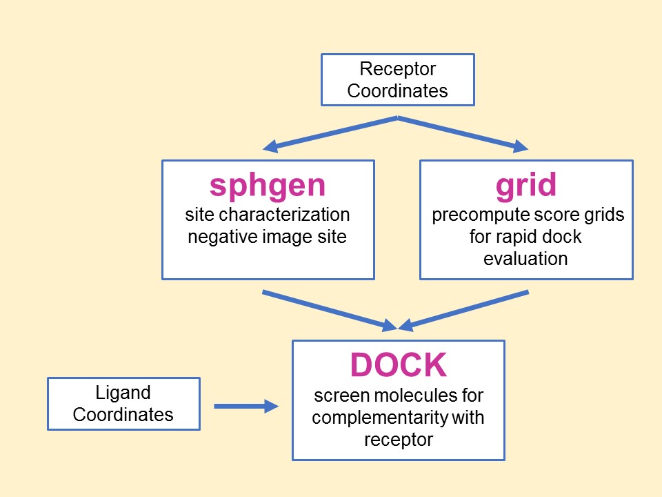
The relationship between the main
programs in the dock suite is depicted in Figure 1. These routines will
be described below.
Main
programs in DOCK suite
The program sphgen
identifies the active site, and other sites of interest, and generates
the sphere centers that fill the site. It has been described in the
original paper (Kuntz et al. J.
Mol. Biol. 1982). The program grid
generates the scoring grids
(Shoichet
et al. J. Comp. Chem. 1992 and
Meng et al. J.
Comp. Chem. 1992). Within the DOCK suite of
programs, the program DOCK matches spheres
(generated by sphgen) with ligand atoms and uses
scoring grids (from grid) to
evaluate ligand orientations (Kuntz
et al. J. Mol. Biol. 1982 and
Shoichet et al. J.
Comp. Chem. 1992). Program DOCK also minimizes
energy based scores (Meng
et al. Proteins 1993).
1.5.2. General Concepts
The DOCK suite of programs is designed to find
favorable orientations of a ligand in a “receptor.”
It can be subdivided into
(i) those programs related directly
to docking of ligands and
(ii) accessory programs.
We limit the discussion in this
section to only
those programs and methods related to docking a ligand in a receptor. A
typical receptor might be an enzyme with a well-defined active site,
though any macromolecule may be used (e.g. a structural protein, a
nucleic acid strand, a “true” receptor).
We’ll use an
enzyme as an example in the rest of this discussion.
The starting point of all docking
calculations is
generally the crystal or NMR structure of an enzyme from an
enzyme-ligand complex. The ligand structure may be taken from the
crystal structure of the enzyme-ligand complex or from a database of
compounds, such as the ZINC database (Irwin, et. al. J.
Chem. Inf. Model. 2005).
The primary consideration in the design of our docking programs has
been to develop methods which are both rapid and reasonably accurate.
These programs can be separated functionally into roughly two parts,
each somewhat independent of the other:
(i) Routines which determine the
orientation of a ligand relative to the receptor and
(ii) Routines which evaluate (score) a ligand orientation.
There is a lot of flexibility. You can generate
orientations outside of DOCK and score them with the DOCK evaluation
functions. Alternatively, you can develop your own scoring routines to
replace the functions supplied with DOCK.
The ligand orientation in a receptor site is broken
down into a series of steps, in different programs. First, a potential
site of interest on the receptor is identified. (Often, the active site
is the site of interest and is known a priori.) Within this site,
points are identified where ligand atoms may be located. A routine from
the DOCK suite of programs identifies these points, called sphere
centers, by generating a set of overlapping spheres which fill the
site. Rather than using DOCK to generate these sphere centers,
important positions within the active site may be identified by some
other mechanism and used by DOCK as sphere centers. For example, the
positions of atoms from the bound ligand may be used as these sphere
centers. Or, a grid may be generated within the site and each grid
point may be considered as a sphere center. Our sphere centers,
however, attempt to capture shape characteristics of the active site
(or site of interest) with a minimum number of points and without the
bias of previously known ligand binding modes.
To orient a ligand within the active
site, some of
the sphere centers are “matched” with ligand atoms.
That
is, a sphere center is “paired” with an ligand
atom. Many
sets of these atom-sphere pairs are generated, each set containing only
a small number of sphere-atom pairs. In order to limit the number of
possible sets of atom-sphere pairs, a longest distance heuristic is
used; (long) inter-sphere distances are roughly equal to the
corresponding (long) inter-atomic ligand distances. A set of
atom-sphere pairs is used to calculate an orientation of the ligand
within the site of interest. The set of sphere-atom pairs which are
used to generate an orientation is often referred to as a match. The
translation vector and rotation matrix which minimizes the rmsd of
(transformed) ligand atoms and matching sphere centers of the
sphere-atom set are calculated and used to orient the entire ligand
within the active site.
The orientation of the ligand is
evaluated with a
shape scoring function and/or a function approximating the
ligand-enzyme binding energy. Most evaluations are done on (scoring)
grids in order to minimize the overall computational time. At each grid
point, the enzyme contributions to the score are stored. That is,
receptor contributions to the score, potentially repetitive and time
consuming, are calculated only once; the appropriate terms are then
simply fetched from memory.
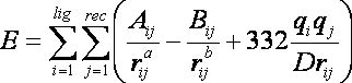
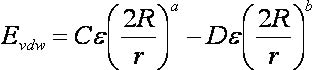
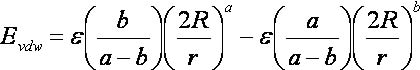
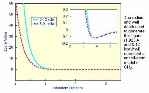
The ligand-enzyme binding energy is
taken to be
approximately the sum of the van der Waals attractive, van der Waals
dispersive, and Coulombic electrostatic energies. Approximations are
made to the usual molecular mechanics attractive and dispersive terms
for use on a grid. To generate the energy score, the ligand atom terms
are combined with the receptor terms from the nearest grid point, or
combined with receptor terms from a “virtual” grid point
with interpolated receptor values. The score is the sum of over all
ligand atoms for these combined terms. In this case, the energy score
is determined by both ligand atom types and ligand atom positions on
the energy grids.
As a final step, in the energy
scoring scheme, the
orientation of the ligand may be varied slightly to minimize the energy
score. That is, after the initial orientation and evaluation (scoring)
of the ligand, a simplex minimization is used to locate the nearest
local energy minimum. The sphere centers themselves are simply
approximations to possible atom locations; the orientations generated
by the sphere-atom pairing, although reasonable, may not be minimal in
energy.
1.5.3. Specific Concepts
(A) Sphere Centers
Spheres are generated to fill the target site.
The sphere centers are putative ligand atom positions. Their use is an
attempt to limit the enormous number of possible orientations within
the active site. Like ligand atoms, these spheres touch the surface of
the molecule and do not intersect the molecule. The spheres are allowed
to intersect other spheres; i.e., they have volumes which overlap. Each
sphere is represented by the coordinates of its center and its radius.
Only the coordinates of the sphere centers are used to orient ligands
within the active site (see above). Sphere radii are used in
clustering.
The number of orientations of the ligand in free
space is vast. The number of orientations possible from all sets of
sphere-atom pairings is smaller but still large and cannot be generated
and evaluated (scored) in a reasonable length of time. Consequently,
various filters are used to eliminate from consideration, before
evaluation, sets of sphere-atoms pairs, which will generate poorly
scoring orientations. That is, only a small subset of the number of
possible ligand orientations are actually generated and scored. The
distance tolerance is one filter. Sphere “coloring”
and
identification of “critical” spheres are other
filters.
Sphere-sphere distances are compared
to atom-atom
distances. Sets of sphere-atom pairs are generated in the following
manner: sphere i is
paired with atom I
if and only if for every sphere j in
the set and for every atom J
in the set,
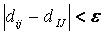
where dij
is the distance between sphere i and sphere
j, dIJ is the
distance between atom I and atom J,
and epsilon is a somewhat small user-defined
value.
(B) Chemical Matching
DOCK spheres are generated without
regard to the
chemical properties of the nearby receptor atoms. Sphere
“chemical matching” or
“coloring” associates a
chemical property to spheres and a sphere of one
“color”
can only be matched with a ligand atom of complementary color. These
chemical properties may be things such as “hydrogen-bond
donor,” “hydrogen-bond acceptor,”
“hydrophobe,”
“electro-positive,”
“electro-negative,” “neutral,”
etc. Neither the
colors themselves, nor the complementarity of the colors, are
determined by the DOCK suite of programs; DOCK simply uses these
labels. With the inclusion of coloring, only ligand atoms with the
appropriate chemical properties are matched to the complementary
colored spheres. It is probably more likely, then, that the orientation
generated will produce a favorable score. Conversely, by excluding
colored spheres from pairing with certain ligand atoms, the number of
(probably) unfavorable orientations which are generated and evaluated
can be reduced. Note that requiring complementarity in matching does
not mean that all ligand atoms will lie in chemically complementary
regions of the enzyme. Rather, only those ligand atoms, when paired
with a colored sphere which is part of the sphere-atom match, will be
guaranteed to be in the chemically complementary region of the enzyme
(provided chirality of the spheres is the same as that of the matching
ligand atoms).
(C) Critical Points
The "critical point" filter requires
that certain spheres be part of the set of sphere-atom pairs used to
orient the ligand (DesJarlais
et al. J. Comput-Aided Molec. Design. 1994).
Designating spheres as critical points forces the ligand to have at
least one atom in that area of the enzyme, where that sphere is
located. This filter may be useful, for example, when it is known that
a ligand must occupy a particular area of an active site. This filter
removes from consideration any orientation that does not guarantee at
least one ligand atom in critical areas of the enzyme (provided
chirality of the spheres is the same as that of the matching ligand
atom).
(D) Bump Filter
After a ligand is oriented within
the active
site, the orientation is evaluated. In an attempt to reduce the total
computational time, after the ligand is oriented in the site, it is
possible to first check whether or not ligand atoms occupy space
already occupied by the receptor. If too many of such
“bumps” are found, then the ligand is likely to
intersect
the receptor even after minimization; consequently, the ligand
orientation is discarded before evaluation.
1.5.4. Units
The units of the DOCK suite of programs
are lengths in angstroms, masses in atomic mass units,
charges in electron charges units, and energies in kcal/mol.
For Amber score internally and on input of charges from a prmtop file
the charges are scaled by
18.2223.
RETURN
TO TABLE OF CONTENTS
DOCK
RETURN TO TABLE OF CONTENTS
2.1. Overview
This section is intended as a
reference manual for
the features of the DOCK Suite of Programs. It is intended to give an
overview of the ideas which form the basis of the DOCK suite of
programs and to detail the available user parameters. It is not
intended to be a substitute for all the papers written on DOCK.
In general, this document is geared towards the
experienced user and introduces new features and concepts in version
6. If you are new to DOCK, we strongly recommend you look at the
tutorials on the DOCK web site at http://dock.compbio.ucsf.edu/DOCK_6/index.htm,
which go into much greater practical detail.
RETURN TO TABLE OF CONTENTS
2.2. History
Version 1.0/1.1
Authors: Robert Sheridan, Renee
DesJarlais, Irwin Kuntz
The program DOCK is an automatic procedure for
docking a molecule into a receptor site. The receptor site is
characterized by centers, which may come from sphgen or any other
source. The molecule being docked is characterized by ligand centers,
which may be its non-hydrogen atoms or volume-filling spheres
calculated in sphgen. The ligand centers and receptor centers are
matched based on comparison of ligand-center/ligand-center and
receptor-center/receptor-center distances. Sets of ligand centers match
sets of receptor centers if all the internal distances match, within a
value of distance_tolerance. Ligand-receptor pairs are added to the set
until at least nodes_minimum pairs have been found. At least three
pairs must be found to uniquely determine a rotation/translation matrix
that will orient the ligand in the receptor site. A least-squares
fitting procedure is used (Ferro
et al. Act. Cryst. A. 1977).
Once an orientation has been found, it is evaluated by any of several
scoring functions. DOCK may be used to explore the binding modes of an
individual molecule, or be used to screen a database of molecules to
identify potential ligands.
Version 2.0
Authors: Brian Shoichet, Dale Bodian, Irwin Kuntz
DOCK version 2.0 was written to give the user
greater control over the thoroughness of the matching procedure, and
thus over the number of orientations found and the CPU time required
(Shoichet et al. J.
Comp. Chem. 1992).
In addition, certain algorithmic shortcomings of earlier versions were
overcome. Versions 2.0 and higher are particularly useful for
macromolecular docking (Shoichet
et al. J. Mol. Biol. 1991)
and applications which demand detailed exploration of ligand binding
modes. In these cases, users are encouraged to run CLUSTER in
conjunction with sphgen and DOCK.
To allow for greater control over
searches of
orientation space, the ligand and receptor centers are pre-organized
according to their internal distances. Starting with any given center,
all the other centers are presorted into “bins”
based on
their distance to the first center. All centers are tried in turn as
“first” positions, and all the points in a bin
which has
been chosen for matching are tried sequentially. Ligand and receptor
bins are chosen for matching when they have the same distance limits
from their respective “first” points. The number of
centers
in each bin determines how many sets of points in the receptor and the
ligand will ultimately be compared. In general, the wider the bins, the
greater the number of orientations generated. Thus, the thoroughness of
the search is under user control.
Version 3.0
Authors: Elaine Meng, Brian Shoichet,
Irwin Kuntz
Version 3.0 retained the matching
features of version 2.0, and introduced options for scoring
(Meng et al. J.
Comp. Chem., 1992).
Besides the simple contact scores mentioned above, one can also obtain
molecular mechanics interaction energies using grid files calculated by
CHEMGRID (which is now superseded by GRID in version 4.0). More
information about the ligand and receptor molecules is required to
perform these higher-level kinds of scoring. Point charges on the
receptor and ligand atoms are needed for electrostatic scoring, and
atom-type information is needed for the van der Waals portion of the
force field score. Input formats (some of them new in version 3.5) are
discussed in various parts of the documentation; one example of a
“complete format” (including point charges and atom
type
information) is SYBYL MOL2 format. Parameterization of the receptor is
discussed in the documentation for CHEMGRID. In DOCK, ligand parameters
are read in along with the coordinates; input formats are described
below. Currently, the options are: contact scoring only, contact
scoring plus Delphi electrostatic scoring, and contact scoring plus
force field scoring. Atom-type information and point charges are not
required for contact scoring only.
Version 3.5
Authors: Mike Connolly, Daniel
Gschwend, Andy Good, Connie Oshiro, Irwin Kuntz
Version 3.5 added several features:
score optimization, degeneracy checking, chemical matching and critical
clustering.
Version 4.0
Authors: Todd Ewing, Irwin Kuntz
Version 4.0 was a major rewrite and update of DOCK
(Ewing et al. 2001 ).
A new matching engine was developed which is more robust, efficient,
and easier to use (Ewing
and Kuntz. J. Comput. Chem. 1997).
Orientational sampling can now be controlled directly by specifying the
number of desired orientations. Additional features include chemical
scoring, chemical screening, and ligand flexibility.
Version 5.0-5.4
Authors: Demetri Moustakas, P. Therese
Lang, Scott Pegg, Scott Brozell, Irwin Kuntz
Version 5 was rewritten in C++ in a modular format,
which allows for easy implementation of new scoring functions, sampling
methods and analysis tools (Moustakas
et al., 2006).
Additional new features include MPI parallelization, exhaustive
orientation searching, improved conformation searching, GB/SA solvation
scoring, and post-screening pose clustering.
(Zou et al. J. Am.
Chem. Soc., 1999)
Version 6.0-6.13
Authors: P. Therese Lang, Demetri Moustakas, Scott Brozell,
Noel Carrascal, Sudipto Mukherjee, Lauren Prentis, Courtney Singleton, Yuchen Zhou,
Brian Fochtman, Trent Balius, T. Dwight McGee Jr.,
William Joseph Allen, John Bickel, Guilherme D. R. Matos, Steven Pak, Christopher Corbo, Brock Boysan, Patrick Holden,
Scott Pegg, Kaushik Raha, Devleena Shivakumar,
Robert Rizzo, David Case, Brian Shoichet, Irwin Kuntz
DOCK 6 is an extension of the DOCK 5 code base. It
includes the implementation of Hawkins-Cramer-Truhlar GB/SA solvation
scoring with salt screening and PB/SA solvation scoring through
OpenEye's Zap Library. Additional flexibility has been added to scoring
options during minimization. The new code also incorporates DOCK
version 3.5.54 scoring features like Delphi electrostatics,
ligand desolvation, and receptor
desolvation. Finally, DOCK 6 introduces new code that allows access to
the NAB library of functions such as receptor flexibility, the full
AMBER molecular mechanics scoring function with implicit solvent,
conjugate gradient minimization, and molecular dynamics simulation
capabilities. DOCK 6 includes searching methods
(DOCK_DN, DOCK_GA) and the ability to create fragment libraries. DOCK_D3N
depends on an enhanced version of DOCK by integrating RDKit.
See
Lang et al. RNA, 2009,
Brozell et al., 2012,
Allen et al., 2015,
Allen et al., 2017,
Prentis et al., 2022,
Matos and Pak et al. 2023, and
Bickel et al. 2025
RETURN TO TABLE OF CONTENTS
2.3.
Command-line Arguments
DOCK must be run from the command line in a standard unix
shell. It reads an input parameter file containing field/value pairs:
USAGE: dock6 -i dock.in [-o dock.out] [-v]
DESCRIPTION:
DOCK may be executed in either interactive or batch mode, depending on
whether the output is written to a file. In interactive mode, the user is
requested only for parameters relevant to the particular run and
default values are provided. This mode is recommended for the initial
construction of the input file and for short calculations. In batch
mode, input parameters are read in from the input file and all output
is written to the output file. This mode is recommended for long
calculations once an input file has been generated interactively.
OPTIONS
-i dock.in #input file containing user-defined parameters
-help #emit the usage statement.
-v #verbosity flag that prints additional
information and warnings for scoring functions
-o dock.out #output file containing the parameters
used in the calculation, summary information for each molecule docked,
and all warning messages
Interactive mode
USAGE: dock6 -i dock.in
DESCRIPTION:
When launched this way, DOCK will extract all
relevant parameters from dock.in (or any file supplied by the user). If
additional parameters are needed (or if the dock.infile is non-existent
or empty), DOCK will request them one at a time from the user.
Reasonable default values are presented. Any parameters supplied by the
user will be automatically appended to the dock.in file. If the user
would like to change any previously entered values, the user can edit
the dock.in file using a text editor.
Batch mode
USAGE: dock6 -i dock.in -o dock.out
DESCRIPTION:
When launched in this way, DOCK will run in batch
mode, extracting all relevant parameters from dock.in (or any file
supplied by the user) and will write out all output to dock.out (or any
file supplied by the user). If any parameters are missing or incorrect,
then execution will halt and an appropriate error message will be
reported in dock.out.
Parallel DOCK
USAGE: mpirun [-machinefile
machfile] [-np #_of_proc] dock6.mpi -i dock.in -o dock.out [-v]
DESCRIPTION:
If DOCK has been built for parallel processing
(see Installation) then
DOCK can be run in parallel.
Parallelization employs
a single master processor with the remaining processors acting as slaves.
If np = 1, the code defaults to non-MPI behavior.
There is a minimal difference in performance between 1 and 2 processors.
Improved performance is only evident with more than 2 processors.
In some MPIs dock6.mpi should be launched with mpiexec.
ADDITIONAL OPTIONS:
-machinefile #simple text
file containing the names of the computers (nodes) to be used
-np # specifies the number of processors which typically is the
same as the number of lines in the machinefile
For additional details on your MPI installation, read the man page:
man mpirun
RETURN TO TABLE OF CONTENTS
2.4. The
Parameter Parser
In Interactive
Mode, dock will dynamically ask the user to enter the
appropriate user parameters. The generic format for the questions is:
parameter_name [default value]
(legal values):
The parameter parser requires that the
values entered for a parameter exactly match one of the legal values.
For example:
Example A: program_location
[Hello_World!] ():
Example B: #_red_balloons [99] ():
Example C: glass_status [half_full]
(half_full half_empty):
In Example A, the parameter
"program_location" can
be assigned any string value, and in Example B, the parameter
"#_red_balloons" can be assigned any integer value. However, in Example
C, the parameter value "glass_status" can only be assigned the strings
"half_full" or "half_empty". If no parameter are assigned by the user,
the default value--in brackets--will be used.
In Batch
Mode, all parameters in the dock.in file, must be:
parameter_name value
Note that the parameter_name and corresponding
value must be separated by white space, namely, blanks or tabs.
RETURN TO TABLE OF
CONTENTS
2.5. Sampling Methods
Before you can dock a ligand, you will need atom
types and charges for every atom in the ligand. Currently, DOCK
reads the Tripos MOL2 format. For a single ligand (or several ligands),
you can use Chimera in combination with antechamber to prepare a MOL2
file for the ligand (see Structure
Preparation Tutorial)
or various other visualization packages. During the docking procedure,
ligands are read in from a single MOL2 or multi-MOL2 file. Atom and
bond types are assigned using the DOCK 4 atom/bond typing parameter files.
For hierarchical database search, dock will read in db2 files which efficiently store multiple ligand conformations.
Many new sampling methods have been fully integrated into DOCK6, where users will be
able to access powerful virtual screening capabilities, from scratch de novo growth
(DOCK_DN), and evolution-based searching (DOCK_GA). We have added hierarchical database search (HDB) which performs hierarchical traversal through precomputed ligand conformations to enable large-scale docking. (Balius, J.Comput. Chem. 2024) We also now have a covalent docking method called attach-and-grow (this method is still in development).
Sampling Method Input Parameter
| Parameter |
Description |
Default Value |
| conformer_search_type |
Choose the type of docking calculation: Rigid body docking (rigid), Flexible ligand docking (flex), de novo ligand design (denovo), Genetic Algorithm ligand construction (genetic), hierarchical database search (HDB), attach-and-grow (covalent) |
flex |
RETURN TO TABLE OF CONTENTS
2.5.1. Rigid and Flexible Ligand Docking
The internal degrees of freedom of the ligand can be sampled
with the anchor-and-grow incremental construction approach.
This conformational search algorithm has been validated
for binding mode prediction using a large dataset derived from the
protein data bank of 1043 protein-ligand complexes
(Allen et al., 2015).
2.5.1.1.
Anchor-and-Grow
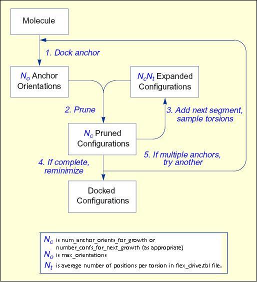
The process of docking a molecule using the
anchor-first strategy is shown in the Workflow for Anchor-and-Grow Algorithm
Ewing et al. 2001 .
First, the largest rigid substructure of the ligand (anchor)
is identified (see
Identification of Rigid Segments) and
rigidly oriented in the active site (orientation) by matching the center of the
heavy atoms to that of the receptor spheres
(see Orienting the Ligand).
The anchor orientations are evaluated and optimized using the scoring
function (see Scoring) and
the energy minimizer (see Minimization).
In general,
the orientations are then ranked according to their score, spatially
clustered by heavy atom root mean squared deviation (RMSD), and pruned
(see Pruning
the Conformation Search Tree). Next, the remaining flexible
portion of the ligand (see
Identification of Flexible Layers)
is built onto the best anchor orientations within the context of the
receptor (grow). It is assumed that the shape of the binding site will
help restrict the sampling of ligand conformations to those that are
most relevant for the receptor geometry.
Workflow
for Anchor-and-Grow Algorithm
Starting with version 6.8,
ligand conformational searching is enabled when the
conformer_search_type input parameter is set to flex.
In versions 6.7 and earlier of DOCK, the corresponding input parameter
was flexible_ligand [yes] (yes no).
Only the torsion
angles are modified, not the bond lengths or angles. Therefore, the
input geometry of the molecule needs to be of good quality. A structure
generated by ZINC15 is sufficient.
The torsion angle positions reside in an editable
file (see flex_drive.tbl on page 111) which is identified with the
flex_drive_file parameter. Internal clashes are detected during the
torsion drive search based on the clash_overlap or internal_energy
parameters, which are independent of scoring function.
RETURN TO TABLE OF CONTENTS
2.5.1.2.
Identification of Rigid Segments
A flexible molecule is treated as a collection of
rigid segments. Each segment contains the largest set of adjacent atoms
separated by non-rotatable bonds. Segments are separated by rotatable
bonds.
The first step in segmentation is ring identification.
All bonds within molecular rings are treated as rigid.
This classification scheme is a first-order approximation of molecular
flexibility, since some amount of flexibility can exist in non-aromatic
rings. To treat such phenomenon as sugar puckering and chair-boat
hexane conformations, the user will need to supply each ring
conformation as a separate input molecule. Additional bonds may be
specified as rigid by the user
(see Manual
Specification of Non-rotatable Bonds).
Identification
of Rigid Anchor and Flexible Bonds
The second step is flexible bond
identification. Each flexible bond is associated with a label defined
in an editable file (see flex.defn).
The parameter file is identified with the flex_definition_file
parameter. Each label in the file contains a definition based on the
atom types (and chemical environment) of the bonded atoms. Each label
is also flagged as minimizable. Typically, bonds with some degree of
double bond character are excluded from minimization so that planarity
is preserved. Each label is also associated with a set of preferred
torsion positions. The location of each flexible bond is used to
partition the molecule into rigid segments. A segment is the largest
local set of atoms that contains only non-flexible bonds.
RETURN TO TABLE OF CONTENTS
2.5.1.3.
Manual Specification of Non-rotatable Bonds
Currently this functionality is not available!
The user can potentially specify additional bonds to be
non-rotatable, to supplement the ring bonds automatically identified by
DOCK. Such a technique could be used to preserve the conformation of
part of a molecule and isolate it from the conformation search.
Non-rotatable bonds are identified in the Tripos MOL2 format file
containing the molecule. The bonds are designated as members of a
STATIC BOND SET named RIGID (see Tripos
MOL2 Format).
Creation of the RIGID set can be done within
Chimera. With the molecule of interest loaded into Chimera, select the
portion of the ligand you would like to remain rigid. Then select on
File > Save MOL2. Make sure the "Write current selection to @
SETS section of file" is checked and save the file.
Alternatively, the RIGID set can be entered into
the MOL2 file by hand. To do this, go to the end of the MOL2 file. If
no sets currently exist, then add a SET identifier on a new line. It
should contain the text "@<TRIPOS>SET". On a new line add
the text "RIGID STATIC BONDS <user> **** Comment". On the
next line
enter the number of bonds that will be included in the set, followed by
the numerical identifier of each bond in the set.
RETURN TO TABLE OF CONTENTS
2.5.1.4.
Identification of Flexible Layers
Anchor Selection
An anchor segment is normally selected from
the rigid segments in an automatic fashion
(see Manual
Specification of Non-rotatable Bonds
to override this behavior). The molecule is divided into segments that
overlap at each rotatable bond. The segment with the largest number of
heavy atoms is selected as the first anchor, number of attachment points are also
considered. All segments with more heavy atoms than min_anchor_size are tried
separately as anchors. The number of anchors can be limited by setting the
limit_max_anchors flag to "yes"; max_anchor_num is used to specify the maximum
number of anchors to be used (anchors are ordered by heavy atoms and attachment
points):
min_anchor_size 5
limit_max_anchors yes
max_anchor_num 5
At most 5 anchors are used and all anchors have at least 5 heavy atoms.
To use a single specific anchor (e.g scaffold with known binding pose), specify an atom name and its corresponding atom number in the chosen fragment (e.g. if atom number 10 is C16):
user_specified_anchor yes
atom_in_anchor C16,10
Identification
of Overlapping Segments
When an anchor has been selected,
then the molecule is redivided into non-overlapping segments, which are
then arranged concentrically about the anchor segment. Segments are
reattached to the anchor according to the innermost layer first and
within a layer to the largest segment first.
Layered
Non-Overlapping Segments
The anchor is processed separately
(either oriented, scored, and/or minimized). The remaining segments are
subsequently re-attached during the conformation search. The
interaction energy between the receptor and the ligand can be optimized
with a simplex minimizer (see Minimization).
RETURN TO TABLE OF CONTENTS
2.5.1.5.
Pruning the Conformation Search Tree
Starting with version 6.1,
there are two methods for pruning.
The first method is the one that existed in earlier versions;
it is the default and corresponds to input parameter
pruning_use_clustering = yes.
In this method
pruning attempts to retain the best, most diverse configurations using
a top-first pruning algorithm, which proceeds as follows. The
configurations are ranked according to score. The top-ranked
configuration is set aside and used as a reference configuration for
the first round of pruning. All remaining configurations are considered
candidates for removal. A root-mean-squared distance (RMSD) between
each candidate and the reference configuration is computed.
Each candidate is then evaluated for removal
based on its rank and RMSD using the inequality:
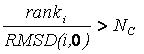
If the factor is greater than
number_confs_for_next_growth, as appropriate, the candidate is removed.
Based on this factor, a configuration with rank 2
and 0.2 angstroms RMSD is comparable to a configuration with rank 20
and 2.0 angstroms RMSD. The next best scoring configuration which
survives the first pass of removal is then set aside and used as a
reference configuration for the second round of pruning, and so on.
This pruning method biases its search time towards molecules that sample a
more diverse set of binding modes. As the values of
num_anchors_orients_for_growth and number_confs_for_next_growth are
increased, the anchor-first method approaches an exhaustive search.
In the second method, the goal is to bias
the sampling towards
conformations that are close to the correct binding mode (as optimized
using a test set of experimentally solved structures). Much as the
method above, the algorithm ranks the generated poses and
conformations. Then, all poses that violate a user-defined score cutoff
are removed. To facilitate the speed of the calculation, the remaining
list is additionally pared back to a user-defined length.
In this method, the sampling is driven towards molecules that sample
closer
to the experimentally determined binding site, and the result is
a significantly less diverse set of final poses.
RETURN TO TABLE OF CONTENTS
2.5.1.6
Time Requirements
The time demand grows linearly with thenumber of anchor segments explored for a given molecule,
num_anchors_orients_for_growth, the
number of flexible bonds and the number of torsion positions per bond, as well as the number_confs_for_next_growth.
Using the notation in the Workflow for
Anchor-and-Grow Algorithm, the time demand can be expressed
as
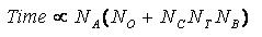
where the
additional terms are:
NA is the number of anchor segments tried per
molecule.
NB is the number of rotatable bonds per molecule.
RETURN TO TABLE OF CONTENTS
2.5.1.7.
Growth Tree and Statistics
Dock uses Breadth First Search to sample the conformational space of the ligand. The tree is pruned at every stage of growth to remove unsuitable conformations. In order to be as space efficient as possible, DOCK only saves one level of growth at a time unless "write_growth_tree" is turned on. In order to construct the growth tree it was necessary to do the following: (1) Retain all levels of growth (before and after minimization) in memory. (2) Link every conformer to its parent conformer during growth. (3) While writing out the tree, the traversal starts from a fully grown ligand (leaf), moving up the branch (parent conformer) until the ligand anchor (root) is reached. Finally, the growth tree branch is printed as a multi-mol2 file starting from the anchor to the fully grown ligand, including minimizations. This newly implemented feature allows visualization of all stages of growth and optimize behavior of current DOCK routines. Note that the growth trees can easily be visualized using the
ViewDock module in the UCSF chimera program. Extra information regarding conformer number, anchor number, parent conformer etc. can also be accessed directly using this tool.
Format for branch files name is as follows:
${Ligand name}_anchor${anchor number}_branch${conformer number of fully grown mol.}.mol2
e.g. LIG1_anchor1_branch4.mol2
The ligand name is that specified in the mol2 file.
The anchor number indicates what fragment or portion of the molecule was used as the anchor.
The every conformer (both partially and fully grown) is assigned a unique number.
we recommend that users cat files together and compress them.
cat *_branch*.mol2 > growth_tree.mol2; gzip growth_tree.mol2
In addition, growth statistics are printed to the output files if the verbose flag is used.
-----------------------------------
VERBOSE MOLECULE STATS
Number of heavy atoms = 30
Number of rotatable bonds = 7
Formal Charge = 1.00
Molecular Weight = 429.56
Heavy Atoms = 30
-----------------------------------
VERBOSE ORIENTING STATS :
Orienting 10 anchor heavy atom centers
Sphere Center Matching Parameters:
tolerance: 0.25; dist_min: 2; min_nodes: 3; max_nodes: 10
Num of cliques generated: 2298
Residual Info:
min residual: 0.0261
median residual: 0.3932
max residual: 0.5000
mean residual: 0.3737
std residual: 0.0935
Node Sizes:
min nodes: 3
max nodes: 4
mean nodes: 3.0070
# of anchor positions: 1000
-----------------------------------
VERBOSE GROWTH STATS : ANCHOR #1
32/1000 anchor orients retained (max 1000) t=9.06s
Lyr 1-1 Segs|Lyr 2-1 Segs|Lyr 3-2 Segs|Lyr 4-2 Segs|Lyr 5-1 Segs|
Lyr:1 Seg:0 Bond:8 : Sampling 6 dihedrals C6(C.ar) C4(C.ar) C3(C.3) C1(C.3)
Lyr:1 Seg:0 24/192 retained, Pruning: 6-score 162-clustered t=10.68s
Lyr:2 Seg:0 Bond:5 : Sampling 3 dihedrals C4(C.ar) C3(C.3) C1(C.3) N1(N.3)
Lyr:2 Seg:0 51/72 retained, Pruning: 21-clustered t=11.38s
Lyr:3 Seg:0 Bond:1 : Sampling 3 dihedrals C3(C.3) C1(C.3) N1(N.3) S1(S.o2)
Lyr:3 Seg:0 105/153 retained, Pruning: 7-score 41-clustered t=13.37s
Lyr:3 Seg:1 Bond:3 : Sampling 6 dihedrals N4(N.am) C2(C.2) C1(C.3) C3(C.3)
Lyr:3 Seg:1 86/630 retained, Pruning: 8-score 536-clustered t=23.93s
Lyr:4 Seg:0 Bond:43 : Sampling 3 dihedrals C16(C.ar) S1(S.o2) N1(N.3) C1(C.3)
Lyr:4 Seg:0 90/258 retained, Pruning: 168-clustered t=28.85s
Lyr:4 Seg:1 Bond:26 : Sampling 2 dihedrals C11(C.3) N4(N.am) C2(C.2) C1(C.3)
Lyr:4 Seg:1 147/180 retained, Pruning: 5-score 28-clustered t=35.28s
Lyr:5 Seg:0 Bond:46 : Sampling 6 dihedrals C17(C.ar) C16(C.ar) S1(S.o2) N1(N.3)
Lyr:5 Seg:0 104/882 retained, Pruning: 15-outside grid 22-score 741-clustered t=77.71s
These are the verbose growth statistics for flexible docking to 1PPH (thrombin). These are printed only when the verbose flag is enabled in the command line. This feature is useful for debugging incomplete growths and other possible issues with the growth routines. This feature is also useful to show progress when docking in larger peptide-like ligands (20+ rotatable bonds) which can take several hours. Cumulative timing in seconds (e.g. t=13.37s) is shown at the end of each line to allow quick profiling of the slowest steps during docking. A separate section is printed for each anchor sampled when using multiple anchors. For anchor #1, the orienting routine produces 1000 orients, and 37 are retained after clustering and minimization. The ligand has 7 rotatable bonds. The second line shows the assignment of layers and segments. For details on the terminology, please consult the DOCK 4 paper. subsequently, two lines of information are printed for each torsion sampled.
Lyr:1 Seg:0 indicates that this is Layer #1 and Segment #0. Layer and segment number starts from zero, and corresponds to the array indices used internally. Bond:8 refers to bond number in the mol2 file read in. "Sampling 6 dihedrals C6(C.ar) C4(C.ar) C3(C.3) C1(C.3)" specifies the exact torsion being sampled. Six dihedral positions are being sampled in this case, as determined by the drive_id in flex_drive.tbl. 21/246 retained means 21 conformers were retained from the 246 conformers generated during growth (41 conformers x 6 dihedral positions = 246 new conformers). The Pruning: section demonstrates how these (246-21) or 225 conformers were pruned: 2 conformers were outside the energy grid, 5 conformers exceeded the score cut-off (see pruning_conformer_score_cutoff) and 218 conformers were clustered. Typically clustering removes the greatest number of conformers during each torsion grown as controlled by the pruning_clustering_cutoff parameter. The reader is encouraged to verify that the number of conformers retained can be calculated as above at each stage of growth. If the growth tree is turned on, the total number of conformers stored in the growth tree are also reported.
RETURN TO TABLE OF CONTENTS
2.5.1.9 Rigid Body and Flexible Ligand Docking Input Parameters
| Parameter |
Description |
Default Value |
| user_specified_anchor |
Will the user specify an anchor file? |
no |
| atom_in_anchor |
If the user specifies an anchor, which atom label in the anchor? |
C1,1 |
| limit_max_anchors |
Will the user limit the maximum number of anchors docked? |
no |
| max_anchor_num |
If the user limits the number - maximum number of anchors allowed |
1 |
| min_anchor_size |
Minimum number of atoms in the anchor |
5 |
| pruning_use_clustering |
Will pruning the conformers use a clustering algorithm? |
yes |
| pruning_max_orients |
How many orients will be generated prior to pruning? |
1000 |
| pruning_clustering_cutoff |
Maximum number of clusterheads retained from pruning |
100 |
| pruning_orient_score_cutoff |
Maximum score allowed for orientation of the anchor (kcal/mol) |
1000.0 |
| pruning_conformer_score_cutoff |
Maximum score allowed for conformers (kcal/mol) |
100.0 |
| pruning_conformer_score_scaling_factor |
Score cutoff scaling factor to increase of reduce the score cutoff as molecules rebuild |
1.0 |
| use_clash_overlap |
Flag to check for overlapping atomic volumes during anchor and grow |
no |
| clash_overlap |
A clash exists id the distance between a pair of atoms is less than the clash overlap times the sum of their atom type radii |
0.5 |
| write_growth_trees |
Generate large growth tree files (increases memory usage - recommended to concatenate and compress growth tree branches) |
no |
RETURN TO TABLE OF CONTENTS
2.5.2
De novo Design
New to DOCK6.9 is a de novo design approach (DOCK_DN)
that can assemble new ligands from a library of smaller fragments in the context
of a receptor binding site. We believe this will be a welcome addition to the DOCK
community for those users looking to construct new ligands "from scratch" or
perform lead refinement in a target binding site.
However, while substantial progress has been made
(see Allen et al and online tutorials), users should
be warned that the new de novo code has numerous features and only a few parameter
combinations have been thoroughly tested. Thus, the default protocols and parameter choices
outlined below should only be taken as a rough guide. Users would be wise to
perform their own de novo tests as the optimal parameter choices for a specific
system, or specific type of de novo experiment, are likely to be system dependent.
DOCK_DN experiments entail two primary processes: (1) fragment library generation followed by (2)
de novo construction. Fragment generation is discussed in more detail in the section titled Fragment Library Generation.
Users have a choice of two types of de novo construction: (1) ligand assembly in which growth is based on anchor positions
that have been oriented (i.e. sampled to the binding site spheres like the standard DOCK 6 Flex protocol,
see Mukherjee et ) or (2) ligand assembly in which growth
is based on a user supplied anchor position (i.e. a known scaffold geometry). The first type is a true "from-scratch" assembly, while
the second type is better suited for lead refinement. The DOCK
distribution contains test case example input files for both types of experiments.
Next, DOCK_DN generates new molecular structures layer-by-layer, in an
iterative growth approach, sampling different fragments from sidechain, linker, and scaffold
libraries (see next section). The overall flowchart for iterative growth can be seen below.
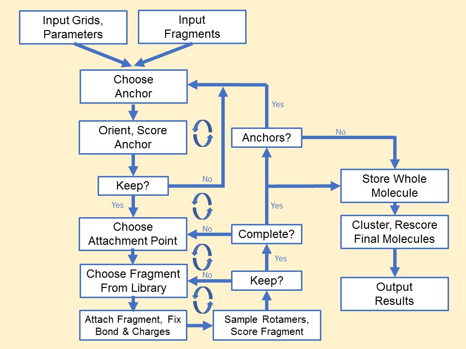
All "complete" molecules, as the growth become completed (no additional
attachment points possible), are written to output files that contain the prefix of
the recently completed layer number. In addition, the final output file contains
all complete molecules that were created over the course of the run. Introduced in DOCK6.12
is a parameter (dn_remove_duplicates) that will write out only one conformer for each
molecule. If users wish to save more conformers, they may turn this parameter off or apply the
associated parameter (dn_max_duplicates_per_mol) to retain more structures on write-out. If this
parameter is turned off and a single unique conformer is desired, users may need to post-process
their results. (see Make Unique Script Usage).
WARNING: Use of de novo design methods, including the genetic algorithm, must include a vdw_defn file that contains parameters for dummy atoms or unintended clashes can occur during growth. This parameter file is included with DOCK6 as vdw_de_novo.defn.
WARNING: The final molecular output files of de novo design are not overwritten at runtime, but are instead appended to as molecules
are built. Users should beware of duplicate structures if experiments are re-run without deletion of output files.
De novo DOCK Refinement
User specified anchor molecules must contain Du atoms to specify attachment points.
This can be done manually in a text based editor such as Vi or Emacs. The screenshot
below shows a modified mol2 file altered to specify attachment of fragments
replacing atom C1. The name of atom C1 has been changed to Du1 and the atom type
has been changed to type Du. For some substitutions additional atoms and bonds may
need to be removed (with bond and atoms counts updated) to generate a structure
maintaining valence properties. To ensure proper valence, bond and atom counts,
structures can be created using a program such as UCSF Chimera, specifying the
attachment point as a rare atom type. The rare atom type can be simply replaced
with Du in a text editor after the structure has been output by Chimera.
	@ TRIPOS ATOM
			1 Du1    1.5994		-16.9463	-11.2883	Du      1	<1>		-0.0418
			2 C2     0.6443		-16.1780	-10.2132	C.ar	1	<1>		-0.1263
			3 C3    -0.4560		-14.9142	-9.8558		C.ar	1	<1>		-0.0990
De novo DOCK Descriptor Driven Design (D3N)
When DOCK is compiled with RDKit (configure with gnu.rdkit or
gnu.parallel.rdkit) termed DOCK/RDKit, DOCK/RDKit takes advantage of multiple cheminformatics
descriptors featured in RDKit. In standard DOCK_DN design, molecules are constructed based on
the user defined energy grids and/or torsion environments. In previous versions, there
was no method to drive molecular construction based on key cheminformatics descriptors,
until now. In version 6.11, users can bias molecular growth to promote partially grown molecules
to the next layers of growth that are contingent on user-defined ranges for the descriptor
being employed. As each partially grown molecule is passed
to the next layer of growth, the molecules undergo a Metropolis-like criteria to assess if the
values for computed descriptors fall within user-defined ranges based on input file.
If they pass the criteria, the molecule is to be sent to the next layer immediately.
However, if molecules fail the criteria, they will be rejected.
Since the criteria is based on Metropolis-like procedure, the resulting distributions
of these descriptors will have soft tails near the user-defined upper and lower limit
for a given ensemble of molecules. Shown below is an example header information for a
constructed molecule. All descriptors that are shown in the descriptor will have a "RD_" prefix.
			##########                   RD_num_arom_rings:                   2
			##########                   RD_num_alip_rings:                   1
			##########                    RD_num_sat_rings:                   0
			##########                    RD_Stereocenters:                   0
			##########                      RD_Spiro_atoms:                   0
			##########                             RD_LogP:            2.505100
			##########                             RD_TPSA:           31.350000
			##########                           RD_SYNTHA:            2.218558
			##########                              RD_QED:            0.798296
			##########                             RD_LogS:           -3.425866
			##########                     RD_num_of_PAINS:                   0
			##########                      RD_PAINS_names:            NO_PAINS
			##########                           RD_SMILES:c1csc(Cc2ccc3c(c2)OCCO3)n1
Fragment and Torsion Biasing
Added in DOCK6.13, methods for biasing the selection and acceptance of fragments as well as the acceptance of torsions was introduced (Bickel J. Comp. Chem.2025). So long as standard library fragmentation is performed, which will result in the FREQ header entry in all fragments and the associated torsions for all torsions in the library, this method will use those frequencies to attempt to shift the ensemble's composition. For Fragment Selection, this will be attempted during selection of a fragment, attempting to select higher frequency fragments more often. For Fragment and Torsion Acceptance, this will be done after selection, providing a chance to "terminate" growth paths that may be less frequent (ie less important, in the case of this method). The below figure outlines how these selections are performed, with a random number deciding the selected fragment and the range of fragments/torsions that would be accepted.
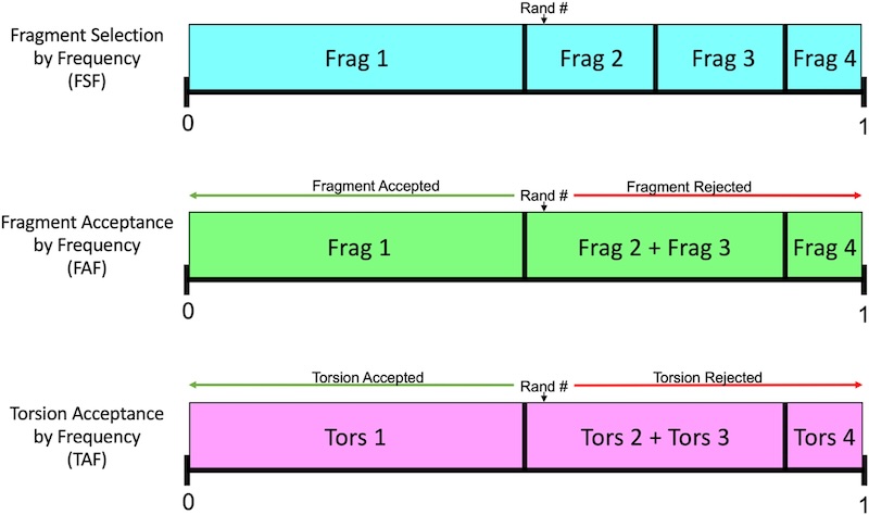
2.5.2.1 DOCK_DN Input Parameters
| Parameter |
Description |
Default Value |
| dn_fraglib_scaffold_file |
The path to the fragment library for just scaffolds |
|
| dn_fraglib_linker_file |
The path to the fragment library for just linkers |
|
| dn_fraglib_sidechain_file |
The path to the fragment library for just side chains |
|
| dn_user_specified_anchor |
Choose whether to provide an anchor (yes), or have DOCK search for an anchor from within the fragment libraries. |
yes |
| dn_fraglib_anchor_file |
The path to the anchor .mol2 file |
|
| dn_use_torenv_table |
Will torsion environment be used? |
yes |
| dn_torenv_table |
The path to the torsion environment (.dat) |
|
| dn_bias_torsions |
Determines if acceptance of torsions by relative frequency after attachment of a fragment will be performed. |
no |
| dn_sampling_method |
Choose which method to use when choosing fragments for each layer (exhaustive, random, graph) |
graph |
| dn_graph_max_picks |
The number of fragment picks per layer per Dummy atom when graph method is turned on |
30 |
| dn_graph_breadth |
The number of fragments that are similar (using Tanimoto) to a successful fragment when graph method is turned on. |
3 |
| dn_graph_depth |
Parameter that controls the overall number of fragment attempted via the following formula: Total_attempts=(max_picks)x=(breadth)^(depth). |
2 |
| dn_graph_temp |
The beginning annealing temperature when graph method is turned on. Higher temperatures lead to greater likelihood of fragment selection even if score does not improve. |
100.0 |
| dn_num_random_picks |
Number of fragments randomly chosen to add to anchor when random method is turned on |
|
| dn_bias_with_fragments |
Determines whether fragment-based biasing will be used. |
no |
| dn_sel_frag_by_freq |
If fragment biasing is enabled, determines whether selection of fragments during growth will be performed. |
no |
| dn_accept_frag_by_freq |
If fragment biasing is enabled, determines whether acceptance of fragments after attachment will be performed. |
no |
| dn_pruning_conformer_score_cutoff |
The max score allowed for fragment conformer addition to be accepted (kcal/mol) if that fragment is in the top (dn_max_layer_size) scoring of each layer. |
100.0 |
| dn_pruning_conformer_score_scaling_factor |
Scaling factor which alters dn_pruning_conformer_score with each layer. Set the scaling factor to 1 then the cutoff stays the same at each layer; set it to 2 and it is halved at each layer. |
2.0 |
| dn_pruning_clustering_cutoff |
Parameter which impacts clustering of anchor orients. The lower value the more anchor orients are kept. |
100.0 |
| dn_remove_duplicates |
Determines whether duplicates of complete molecules are removed at the end of growth, based on Tanimoto. |
yes |
| dn_max_duplicates_per_mol |
Specifies the number of molecules to be kept in the ensemble - defaulted to no duplicates. |
0 |
| dn_write_pruned_duplicates |
If turned on, any duplicates that are pruned by Tanimoto will be written to their own file. |
no |
| dn_advanced_pruning |
Master parameter for advanced pruning. |
yes |
| dn_prune_initial_sample |
Controls pruning of the initial attachments performed on a growing molecule |
yes |
| dn_sample_torsions |
Controls whether or not torsions are sampled. Constructing with internal energy only as the scoring function is the major reason to turn this off. |
yes |
| dn_prune_individual_torsions |
Controls pruning of each individual torsional sampling. Each growing molecule will have all of its potential growth paths pruned for each individual attempted attachment. |
yes |
| dn_prune_combined_torsions |
Controls ensemble pruning for each attachment point. This is performed after all attachments for a given attachment point have been attempted and all torsions sampled. |
yes |
| dn_random_root_selection |
Controls whether or not roots for the next layer will be selected randomly, rather than the best by scoring function. Constructing with internal energy only as the scoring function is the major reason to turn this off. |
no |
| dn_mol_wt_cutoff_type |
Parameter which determines the use of a "hard" upper and lower cutoff for molecular weight (no molecules beyond those values) or a "soft" cutoff (accepted based on standard deviation). |
soft |
| dn_upper_constraint_mol_wt |
The max molecular weight allowed, or the upper boundary before the standard deviation is assessed. |
550 |
| dn_lower_constraint_mol_wt |
The minimum molecular weight allowed, or the lower boundary before the standard deviation is assessed. |
0 |
| dn_mol_wt_std_dev |
If using a soft molecular weight cutoff, this is the standard deviation that determines the probability of acceptance beyond the cutoffs. |
35.0 |
| dn_constraint_rot_bon |
The max rotatable bonds allowed |
15 |
| dn_constraint_formal_charge |
Largest absolute charge of molecule |
2.0 |
| dn_heur_unmatched_num |
# of unmatched heavy atoms for hRMSD to be considered a different molecule when pruning between root and layer |
1 |
| dn_heur_matched_rmsd |
Max rmsd of matching heavy atoms of molecules to be considered similar molecule when pruning root to layer |
2.0 |
| dn_unique_anchors |
The number of unique anchors post clustering |
3 |
| dn_max_grow_layers |
The maximum number of layers that can be grown from a given starting anchor. |
9 |
| dn_max_root_size |
The number of new anchors that seed the next layer of growth |
25 |
| dn_max_layer_size |
The number of partially grown molecules that advance through the search to subsequent attachment points |
25 |
| dn_max_current_aps |
Maximum attachment points the molecule can have at any one time (stop adding new scaffolds when the current fragment has this many open attachment points) |
5 |
| dn_max_scaffolds_per_layer |
The max number of scaffolds added per layer per molecule |
1 |
| dn_write_checkpoints |
Write molecules for each layer |
yes |
| dn_write_prune_dump |
Write all molecules pruned out at every step (large memory output) |
yes |
| dn_write_orients |
Write out the orients |
no |
| dn_write_growth_trees |
Shows growth for every accepted molecule (may produce large output files) |
no |
| dn_output_prefix |
The prefix of the output file with final molecules |
output |
DOCK_DN Output Components
In the 6.12 release, The output of the DOCK_DN method has been overhauled. Below is an example portion of the new output, where the given run has finished Layer 8.
``` dn.out
1  ##### Entering layer of growth #8
2  Root size at the beginning of this layer = 6
3    In Root [ 0], sccf atts 322 |acc mols 98 |cmpd 59 |fltrd cmpd 59 |Prnd 39 |Kpt 0 |S 16.83|A/S 19.13
4    In Root [ 1], sccf atts 413 |acc mols 98 |cmpd 47 |fltrd cmpd 47 |Prnd 51 |Kpt 0 |S 24.50|A/S 16.85
5    In Root [ 2], sccf atts 297 |acc mols 101|cmpd 30 |fltrd cmpd 30 |Prnd 71 |Kpt 0 |S 16.02|A/S 18.54
6    In Root [ 3], sccf atts 390 |acc mols 83 |cmpd 39 |fltrd cmpd 38 |Prnd 44 |Kpt 0 |S 21.97|A/S 17.75
7    In Root [ 4], sccf atts 168 |acc mols 33 |cmpd 24 |fltrd cmpd 25 |Prnd 9  |Kpt 0 |S 10.97|A/S 15.32
8    In Root [ 5], sccf atts 28  |acc mols 0  |cmpd 0  |fltrd cmpd 0  |Prnd 0  |Kpt 0 |S  3.90|A/S 7.18
9      From all attachments events, 1618 fragments were collected in layer 8 prior to all pruning/filtering.
10      From accepted frags ( N= 413 ) in layer 8,
11          Collected a total of 0 candidate root fragments, then that number goes down to 0 due to pruning by the RMSD heuristic.
12          -------------------------------------------
13          0    duplicate fragments were found.
14          199  complete molecules were filtered
15          214  root fragments were filtered
16          0    completed molecules were written to file
17          -------------------------------------------
18          0    root frags intended for the next layer were further pruned via rmsd.
19          0    candidate root frags intended for the next layer were ignored due to limit on root size.
20          For prune_root frags, 17 frags couldn't be written out due to failed H-capping protocol
21                                        1 frags couldn't be written out due to failed torsion checks on H-caps.
22
23      Layer 8 completed! Moving on the next layer with 0 root fragments.
24      For Layer 8, time duration is: 94.20 seconds with 17.18 with attachments per second.
```
Lines 3 to 8 shows the basic break down on how many attachments there are per working root
molecule. The following columns show more details on each attachment type. Those columns definitions are
shown below:
DEFINITONS:
sccf atts: number of successful attachments.

acc mols: number of accepted attachments after pruning.

cmpd: number of completed number generated.

fltrd cmpd: number of completed molecule that were filtered based on Molecular Weight, Formal Charge, and Number of Rotatable Bonds.

Prnd: number of partially grown molecules that were pruned due to the limit set by dn_max_layer_size.

Kpt: number of partially grown molecules kept during the growth iterations via sampling the root.

S: how many seconds it took to run for a given root sampling.

A/S: The number of successful attachments per second.
Lines 9 to 21 outline the statistics on how many molecules were written out and
how many were further filtered for an easier understanding on how DOCK_DN is behaving.
Lines 13 to 21 displays the number of molecules that were written out and more details on why
some molecules are not eligible for a write out. Further, the write out system of pruned molecules
has been changed to be more comprehensive. Below shows the types of output .mol2 files that are
written out on-the-fly.
{#} represents anchor number and {##} represents the layer number they have been outputted
|
Details |
Filtering and Pruning Reasons |
|
Nomenclature
|
Finalized with?
|
Partially grown?
|
Valid molecules?
|
Prune via size max Layer
|
Filter via MW/ROT/FC
|
Prune via size of max Root
|
PruneRMSD via hRMSD
|
Output .mol2 nomenclature
|
| Completed |
Sidechains |
N |
Y |
N/A |
Pass |
N/A |
N/A |
output.completed.denovo_build.mol2 |
| Completed: Filtered |
Sidechains |
N |
Y |
N/A |
Failed |
N/A |
N/A |
${output}.anchor_{#}.filtered_comp_layer_{##}.mol2 |
| Pruned via Root |
Hydrogens |
Y |
Y |
Failed |
Failed |
N/A |
N/A |
${output}.anchor_{#}.prune_root_layer_{##}.mol2 |
| Pruned via RMSD |
Hydrogens |
Y |
Y |
N/A |
N/A |
N/A |
Failed |
${output}.anchor_{#}.prune_rmsd_mw_layer_{##}.mol2 |
| Ignored Candidate Root |
Hydrogens |
Y |
Y |
N/A |
N/A |
Failed |
N/A |
${output}.anchor_{#}.cand_root_ign_layer_{##}.mol2 |
| Propagated Root |
Attachment Points |
Y |
N |
N/A |
N/A |
N/A |
N/A |
${output}.anchor_{#}.root_layer_{##}.mol2 |
2.5.2.2 DOCK_D3N Input Parameters
DOCK_D3N is developed on top of DOCK_DN. The input parameters shown below is also prompted with the input parameters in standard
DOCK_DN, when DOCK is compiled with RDKit
| Parameter |
Description |
Default Value |
| dn_drive_verbose |
Turn on verbose D3N to output more information |
no |
| dn_save_all_molecules |
Save all molecules that are rejected by D3N |
no |
| dn_drive_clogp |
Turn on if you want to bias construction with cLogP |
no |
| dn_lower_clogp |
Lower limit of the range |
-0.30 |
| dn_upper_clogp |
Upper limit of the range |
3.75 |
| dn_clogp_std_dev |
Standard deviation of the Metropolis-like procedure |
2.02 |
| dn_drive_esol |
Turn on if you want to bias construction with ESOL(LogS) |
no |
| dn_lower_esol |
Lower limit of the range |
-5.23 |
| dn_upper_esol |
Upper limit of the range |
-1.35 |
| dn_esol_std_dev |
Standard deviation of the Metropolis-like procedure |
1.94 |
| dn_drive_tpsa |
Turn on if you want to bias construction with TPSA |
no |
| dn_lower_tpsa |
Lower limit of the range |
28.53 |
| dn_upper_tpsa |
Upper limit of the range |
113.20 |
| dn_tpsa_std_dev |
Standard deviation of the Metropolis-like procedure |
42.33 |
| dn_drive_qed |
Turn on if you want to bias construction with QED |
no |
| dn_lower_qed |
Lower limit of the range |
0.61 |
| dn_qed_std_dev |
Standard deviation of the Metropolis-like procedure |
0.19 |
| dn_drive_sa |
Turn on if you want to bias construction with Synthetic Accessibility (SynthA/sa) |
no |
| dn_upper_sa |
Upper limit of the range |
3.34 |
| dn_sa_std_dev |
Standard deviation of the Metropolis-like procedure |
0.9 |
| dn_drive_stereocenters |
Turn on if you want to bias construction with number of stereocenters |
no |
| dn_upper_stereocenter |
Upper limit of the range |
2 |
| dn_drive_pains |
Turn on if you want to bias construction with number of Pan-assay Interference Compounds (PAINS/pains) |
no |
| dn_upper_pains |
Upper limit of the range |
1 |
| dn_start_at_layer |
Layer number you want to start D3N |
1 |
| sa_fraglib_path |
Path to SynthA parameters |
sa_fraglib_path |
| PAINS_path |
Path to PAINS parameters |
pains_table_2019_09_01.dat |
NOTE: some descriptors do not have double-sided limits. This is as intended because these descriptors
have a one-sided direction of "most favorable" score.
DOCK_D3N Output Components
1. ${output}.denovo_build.mol2 is the mol2 file containing the complete top scoring molecules. Molecules are
appended to this file as molecules are built to completion.
2. ${output}.denovo_rejected.mol2 is the mol2 file containing the partially/complete
molecules. Whenever molecules are rejected by the Metropolis-like criteria, molecules
will go here. (This file is created, when "dn_save_all_molecules" is turned on. )
3. ${output}.anchor_{#}.root_layer_{##}.mol2 is the partial molecules for each
anchor (#) at each layer (##). These files are generated as the algorithm is running. This feature is
turned on/off by the input parameter "dn_write_checkpoints".
4. ${output}.anchor_{#}.prune_dump_layer_{##}.mol2 is the partial and complete
molecules that were filtered out for having undesirable properties
for each anchor (#) at each layer (##) of growth. This feature is turned on/off by the
input parameter "dn_write_prune_dump".
RETURN TO TABLE OF CONTENTS
2.5.3
DOCK_GA: Small Molecule Evolution using a Genetic Algorithm
Introduced in DOCK6.10 is a genetic algorithm (DOCK_GA) - a molecular
construction method that utilizes evolutionary principles,
including molecular recombination (referred to as crossover), mutation, and natural selection,
to guide de novo design of ligands that interact favorably with the target
(see Prentis et al. and
online tutorials).
DOCK_GA can be used (1) to generate structural analogs with tailored interactions to the
target, (2) as a de novo design method to grow molecules from a molecular segment, and
(3) as a compliment to a screen to identify the
key molecular functionality of that can be used to target the site.
To initiate a DOCK_GA run,a pre-docked molecular or fragment ensemble is required. During
DOCK_GA preparation, fitness pressures are
applied to the initial parent ensemble and structurally similar molecules are removed.
Next, the initial parent ensemble, as well as all subsequent parent ensembles,
undergo crossover to generate offspring followed by mutation of the offspring and the
parents (if the user so chooses). All newly constructed molecules have their energetic
interactions optimized with the receptor through minimization and are subjected to the
fitness pressures, molecular descriptor filters, and bond environment filter. Next, a
subset of the current generation's parents and offspring are selected to become the
parents for the next generation. The aforementioned processes continue until the
maximum number of generations is reached.
Genetic Algorithm Crossovers
Parental crossover occurs between two molecules with overlapping
rotatable bonds in 3D space within the context of the binding site. Molecule pairs
are permitted to undergo single-point crossover, where the substructures on either
side of the overlapping bond are exchanged, generating two offspring. Two versions
of the crossover method, exhaustive and random, have been implemented, where either
all or a randomly selected subset of parents undergo crossover. For both methods,
the distance and angle between parent-parent bond pairs is used to limit mating to
a confined geometric area, thereby promoting the generation of offspring with
reasonable geometries.
Genetic Algorithm Mutations
There are four
types of fragment-based mutations employed in DOCK_GA: addition, deletion,
substitution, or replacement of a portion of the molecule. A subset of offspring (and parents, if specified by user) undergo
fragment-based mutation until the number of mutants reaches the user-defined target
or the maximum mutation attempts is performed. These mutations
allow the ensembles to change in size and composition, including scaffold-hopping behavior
within single segment/fragment structures.
If the initial ensemble is comprised
of one molecule or a group of molecules that do not overlap in the binding site,
parent mutation is required to produce offspring during the first generation.
When a randomly selected molecule undergoes mutation and the product successfully
passes the bond environment filter (torsion environment table), it is prohibited
from producing additional mutants during the current generation.
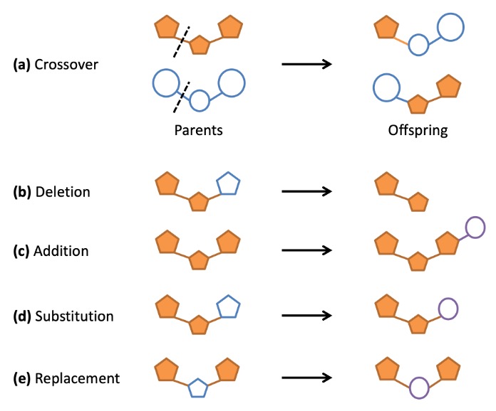
Genetic Algorithm Fitness Function
In preparation for molecule selection, compounds are prioritized
for retention using the fitness function, which is comprised of any user-defined
combination of DOCK6 scoring methods. The score components can be combined linearly
(using the Descriptor Score)
or normalized by the scores present in the current ensemble, using one of the two
niching options discussed later.
Genetic Algorithm Selection
To focus the combinatorial explosions that occurs in de novo design,
molecules are selected at each generation to become the next
generation's parents. This process is performed through one of three selection methods: elitism, roulette,
and tournament. Elitism maintains a user-defined number of the top scoring
molecules. Tournament selection maintains the best scored molecule from a randomly
selected pair of compounds. The roulette method selects molecules based on a
probability function, whereby those with greater fitness are more likely to be
propagated to the next generation.
Both elitism and roulette methods can be executed on the parents and offspring
independently (separate) or the combined ensemble (combined). Tournament selection
can be performed by creating parent-offspring pairs or pairs within each ensemble.
2.5.3.1 DOCK_GA Input Parameters
| Parameter |
Description |
Default Value |
| ga_molecule_file |
Initial molecule ensemble in mol2 format |
ga_molecule_file.mol2 |
| ga_utilities |
Use of GA utilities for this run |
no |
| ga_fraglib_scaffold_file |
Fragment library mol2 file containing scaffolds |
fraglib_scaffold.mol2 |
| ga_fraglib_linker_file |
Fragment library mol2 file containing linkers |
fraglib_linker.mol2 |
| ga_fraglib_sidechain_file |
Fragment library mol2 file containing sidechains |
fraglib_sidechain.mol2 |
| ga_torenv_table |
Path to the torsion environment table (.dat) |
fraglib_torenv.mol2 |
| ga_max_generations |
Max number of generations to be executed |
100 |
| ga_xover_sampling_method_rand |
Selects the random or exhaustive crossover sampling methods (yes for random) |
yes |
| ga_xover_max |
Max number of offspring generated from crossover events |
150 |
| ga_bond_tolerance |
User-specified cutoff for allowable atom sq dist |
0.5 |
| ga_angle_cutoff |
User-specified cutoff for bond angles |
0.14 |
| ga_check_overlap |
Output parent pairs involved in crossover in unique_xover.mol2 file. |
no |
| ga_check_only |
Only check parent pairs for crossover (no offspring, mutations, or selection). |
no |
| ga_add_rate |
% out of 100 of mutation attempts which will be additions |
25 |
| ga_del_rate |
% out of 100 of mutation attempts which will be deletions |
25 |
| ga_sub_rate |
% out of 100 of mutation attempts which will be substitutions |
25 |
| ga_rep_rate |
% out of 100 of mutation attempts which will be replacements |
25 |
| ga_mutate_parents |
Mutate the parents |
no |
| ga_pmut_rate |
Parent mutation rate - only used when random parent mutation is turned on |
0.3 |
| ga_omut_rate |
Offspring mutation rate for random mutation sampling |
0.7 |
| ga_max_mut_cycles |
Max mutation attempts - for random mutation sampling |
5 |
| ga_num_random_picks |
Number of random picks for random sampling |
15 |
| ga_max_root_size |
Max root size in de novo DOCK |
5 |
| ga_energy_cutoff |
The upper bounds for energy pruning |
100 |
| ga_heur_unmatched_num |
The number of unmatched atoms for hRMSD pruning |
1 |
| ga_heur_matched_rmsd |
The RMSD of matched atoms for hRMSD pruning |
0.5 |
| ga_mol_wt_cutoff_type |
Hard or soft MW fitering |
hard |
| ga_constraint_upper_mol_wt |
Upper limit of MW filter |
500.0 |
| ga_constraint_lower_mol_wt |
Lower limit of MW filter |
0.0 |
| ga_constraint_mol_wt_std_dev |
If soft MW filter is set, set standard deviation |
35.0 |
| ga_constraint_rot_bon |
The upper bound for # rot bonds |
10 |
| ga_constraint_H_accept |
The upper bound for # of hydrogen acceptors |
10 |
| ga_constraint_H_donor |
The upper bound for # of hydrogen donors |
5 |
| ga_constraint_formal_charge |
The upper and lower bound for formal charge |
2 |
| ga_ensemble_size |
The number of survivors to carry to next generation |
200 |
| ga_selection_method |
The type of selection (elitism, tournament, roulette) |
elitism |
| ga_elitism_combined |
Combine the parent and offspring populations for the elitism selection method? |
yes |
| ga_elitism_option |
Type of selection:max, percent (perc), or number(num) when elitism is the selection method |
max |
| ga_elitism_number |
The number of top scored parents to pass to the next generation when elitism number is the selection method |
20 |
| ga_elitism_percent |
The top percent of the ensemble(s) to be carried to the next generation when elitism percent is the selection method |
0.2 |
| ga_tournament_p_vs_c |
Select the top scored molecules between parents and offspring separately when tournament selection method is used |
yes |
| ga_roulette_separate |
Select the top scored molecule between parents and offspring separately when roulette selection method is used |
yes |
| ga_max_num_gen_with_no_crossover |
The max number of generations where crossover is not necessary for continuing evolution. After that generation without crossover the algorithm terminates. |
25 |
| ga_name_identifier |
Molecule names prefix in the output files |
ga |
| ga_output_prefix |
Output file name prefix |
ga_output |
DOCK_GA Output Components
1. ${ga_output_prefix}.restart0000.mol2 is the initial parent ensemble to begin DOCK_GA sampling.
2. ${ga_output_prefix}.restart####.mol2 is the molecules from each generation (####). This file can be used as a restart file where the user only needs to
change simplex_random_seed to the number of the generation last completed.
2.5.3.2 DOCK_GA RDKit Input Parameters
When RDKit is compiled with DOCK, the input parameters below will be prompted.
All molecules in the output mol2 files will contain RDKit descriptors in the header.
Currently, DOCK_GA does not have descriptor-driven capabilities.
| Parameter |
Description |
Default Value |
| sa_fraglib_path |
Path to SynthA parameters |
sa_fraglib.dat |
| PAINS_path |
Path to PAINS parameters |
pains_table_2019_09_01.dat |
RETURN TO TABLE OF CONTENTS
2.5.4. Hierarchical DataBase (HDB) Search
For the hierarchical database (HDB) search routine, we precompute molecule conformations, store the conformations in a DB2 file (Coleman, Plos One 2013; Balius, J.Comput. Chem. 2024) with a defined format, read these DB2 files in DOCK, and orient and search through these conformations to find the best scoring poses. For more information about HDB search see Balius et al. (Balius, J.Comput. Chem. 2024). This was implemented to mimic DOCK 3.7 and to enable large scale docking with DOCK 6. DB2 files can be downloaded from the ZINC database (zinc22;zinc20).
Example scripts for building DB2 files can be found here: "[DOCK6path]/template_pipeline/hdb_lig_gen/"
To use HDB set conformer_search_type to HDB.
2.5.4.1 HDB Input Parameters
| Parameter |
Description |
Default Value |
| num_per_search |
Number of poses kept for each orient. The HDB hierarchy is oriented, and then the hierarchy is searched, and a user-specified number of poses are kept. (If the minimizer is turned on, these poses are all minimized.) |
1 |
| skip_broken |
If atoms within a conformation (a branch in the hierarchy) are too close, the conformation is flagged as broken in the DB2 file. If this parameter is "yes", these conformations are skipped. |
no |
| hdb_db2_input_file |
This parameter is for reading in DB2 files. The parameter can take a split_database_index file (as in DOCK 3), which contains a list of db2.gz files; or the parameter can take a single db2.gz file. |
sdi.txt |
| hdb_db2_search_score_threshold |
This is the score cutoff for each segment of the branch. If the score-cutoff is exceeded, then the segment is flagged and all branches containing the segment are halted. (for Grid score and ChemGrid score only VDW term is considered.) |
10.0 |
RETURN TO TABLE OF CONTENTS
2.5.5. Covalent Attach-and-Grow.
Covalent docking can be performed in DOCK6 with the attach-and-grow method (This method is still in development. Use with caution). Attach-and-grow requires two dummy atoms attached to the ligand atom involved in the covalent bond. Attach-and-grow should only be run with the torsion pre-minimizer (the regular minimizer will allow the molecule including the attachment point to move which is undesirable). It uses three spheres to define the attachment location on the receptor. For a cysteine residue these spheres correspond to SG, CB, CA. The dummy atoms are aligned to these spheres. The bond environment is defined by exploring the bondlength, bondlength2 and angle. The dihedral is also sampled. The ligand internal degrees of freedom are explored in the same way as in anchor-and-grow (using the grow periphery functionality).
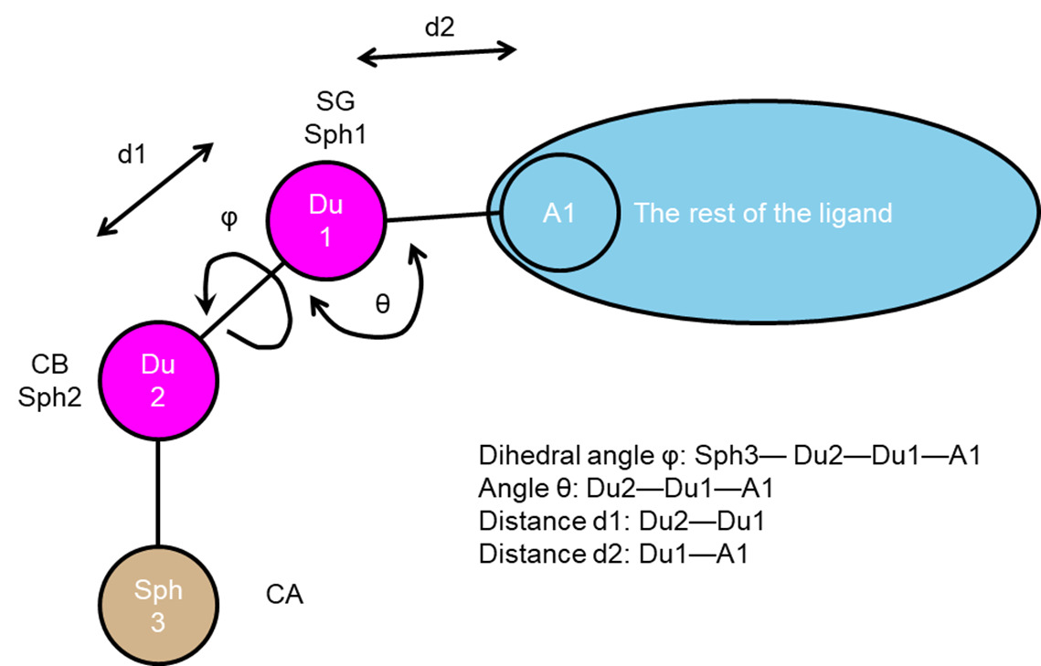
To use attach-and-grow set conformer_search_type to covalent.
2.5.5.1 Covalent Input Parameters
| Parameter |
Description |
Default Value |
| covalent_bondlength |
This defines the bond length between dummy1 (SG) and dummy2 (CB). The user can give a value, or define a range of values. start:step:stop or start:stop (assumes a step size of 0.1). |
1.8 |
| covalent_bondlength2 |
This defines the bond length between dummy1 (SG) and the ligand atom attachment point. The user can give a value, or define a range of values. start:step:stop or start:stop (assumes a step size of 0.1). A value of -1 will use the bond length of the input structure. |
-1 |
| covalent_angle |
This defines the angle between dummy2 (CB), dummy1 (SG) and the ligand atom attachment point. The user can give a value, or define a range of values. start:step:stop or start:stop (assumes a step size of 0.1). A value of -1 will use the angle of the input structure. |
-1 |
| covalent_dihedral_step |
Parameter that defines the dihedral step size (0 to 360). The dihedral is defined by sphere 3(CA), dummy2 (CB), dummy1 (SG) and the ligand atom attachment point. a value of 10 means that 36 dihedral are explored. |
10 |
RETURN TO TABLE OF CONTENTS
2.6.
Fragment Library Generation
Fragments represent the smallest rigid chemical unit perceived by
the program DOCK. These rigid units are determined by the Sybyl atom types of input
molecules and settings in the flexible definition library (flex.defn) distributed
with the program. As a rule, fragments themselves contain no internal
rotatable bonds, however there are some exceptions. For example, methyl, cyano,
halogen, and hydrogen groups are, strictly speaking, rotatable groups. But, rotating
about the R-X bond does not change the nature of the interaction with the receptor.
Thus, these bonds are treated as rigid in the fragment generation process.
In addition, double bonds such as those in alkenes (-C=C-) is not typically
described as a rotatable bond, but de novo DOCK treats it as such with two possible states: cis
and trans. Thus, all double bonds are broken in the fragment generation process.
To generate fragments, molecules in the mol2 format must first be downloaded from a
chemical catalog. The input molecule file is read by de novo DOCK, the molecules are broken at each rotatable bond, and finally fragments are written to file with dummy atoms (labeled as Du)
used as placeholders to mark where the fragment was cleaved. These points in the
fragments, called attachment points, define where two fragments can be connected.
Final fragments are written to three separate output mol2 files, classified as
either sidechains (one attachment point), linkers (two attachment points), or
scaffolds (three or more attachment points). Furthermore, redundant fragments are
removed, and the frequency of each fragment is the input database is recorded in
the header section of the mol2 file. In addition, user may manually add their
preferred fragments to the fragment library. The fragments need to be created following the
rules described above, and be added to the corresponding classification depending
on the number of dummy atoms within each fragment. Users should note that during development we tested MOL2 files from ZINC, MOE, and AMBER.
The MOL2 atom types in particular will influence how the fragments are created. Users should check their MOL2 files prior to fragment library generation,
for example using the view dock feature in UCSF Chimera.
Fragment Visualization
DOCK6.10 introduced a change in how fragments can be output for
better visualization. Using the fragment_library_trans_origin parameter
will both translate all output fragments to the origin, as well as attempt to rotate
them in such a way that major functionality is in the same plane. This does not affect
usage of the fragments in DOCK itself, and is only for manual inspection of the fragment
library in the user's favorite visualization software.
Torsion Environments
For every atom in a given molecule, its local topology in all
directions one bond away is computed and stored as a canonical string. The atom
hybridization, as well as the bond order are considered in these environments, and
the collection of all atom environments in a molecule constitutes its fingerprint.
The application of atom environments to synthetic feasibility becomes clear upon
mining large databases of synthesized, drug-like molecules.
In DOCK, we restrict the formation of new connections to torsion environments that
have been directly observed in databases of existing chemical matter. This is
achieved through an input look-up table provided as a parameter file
(prefix_torenv.dat). These look-up tables are distributed with DOCK, or
can be generated on-the-fly along with fragments as previously described. If the user
chooses to add fragments to the library manually, then the torsion environment table
may also need to be updated to allow connections involving the added fragments. The fragment
library entries can be edited as follows. Using the combine_torenv.py script (located in the bin directory upon compilation), the user can
combine two torsion environments .dat files. This is necessary to increase the likelihood
of success for DOCK_GA runs. The combine_torenv.py requires two files as arguments
combine, sort and remove redundancies to make a master torsion environment table.
DOCK_GA Torsion Environments
DOCK_GA requires a specialized torsion environment table that
includes the bond types of the initial molecules in order to succeed. The torsion
environment table is alphanumerically ordered. The user can use the
combine_torenv.py script located in the bin directory upon compilation to combine multiple
torsion environment tables. Doing so will increase the likelihood of successful
mutations during the genetic algorithm routine.
2.6.1 Fragment Library Generation Parameters
Under current DOCK infrastructure, to write a new fragment library, conformer_search_type must be set to flex.
| Parameter |
Description |
Default Value |
| write_fragment_libraries |
Does the user want to write fragment libraries? (By default, set to no. Must be 'yes' to write libraries) |
no |
| fragment_library_prefix |
Choose a prefix for fragment library file |
fraglib |
| fragment_library_sort_method |
Choose from frequency (freq) or fingerprint (fingerprint) for sorting the fragment library, when fragment library is turned on |
freq |
| fragment_library_trans_origin |
Translate all fragments to a single origin point (no: fragments remain in their original positioning in 3D space) |
yes |
| fragment_library_freq_cutoff |
When frequency fragment library is turned on then what is the minimum frequency allowed in the fragment library? (1 = all fragments allowed) |
1 |
Fragment Library Generation Output Components
1. ${fragment_library_prefix}_sidechain.mol2 is the sidechain fragments file - these fragments contain 1 point of attachment.
2. ${fragment_library_prefix}_linker.mol2 is the linker fragments file - these fragments contain 2 points of attachment.
3. ${fragment_library_prefix}_scaffold.mol2 is the scaffold fragment file - these fragments contain 3 or more points of attachment.
3. ${fragment_library_prefix}_rigid.mol2 is the rigid fragment file, which contains whole molecules lacking any DOCK rotatable bonds.
4. ${fragment_library_prefix}_torenv.dat is the torsion environment table listing all seen bond connections.
RETURN TO TABLE OF CONTENTS
2.7.
Database Filter
The Database Filter is designed for on-the-fly filtering of small molecules from the database during docking. Filtering small molecules by heavy atoms, rotatable bonds, molecular weight and formal charge is currently supported. This routine is designed to be modular so that other descriptors can be easily added. The default values are deliberately set to allow most small molecules to pass through. One use of this routine would be to partition a database into subsets such as "0-7 rotbonds" or "300-500 molwt" or "neutral charge". Another use would be to exclude ligands that are too small (<200 amu) or too large (>500 amu) for a particular target. This routine can also be used to filter a database without performing any docking.
2.7.1 Database Filter Parameters
| Parameter |
Description |
Default Value |
| use_database_filter |
Does the user want to use database filter? |
no |
| dbfilter_max_heavy_atoms |
Maximum number of ligand heavy atoms |
999 |
| dbfilter_min_heavy_atoms |
Minimum number of ligand heavy atoms |
0 |
| dbfilter_max_rot_bonds |
Maximum number of ligand rotatable bonds |
999 |
| dbfilter_min_rot_bonds |
Minimum number of ligand rotatable bonds |
0 |
| dbfilter_max_molwt |
Maximum ligand molecular weight |
9999.0 |
| dbfilter_min_molwt |
Minimum ligand molecular weight |
0.0 |
| dbfilter_max_formal_charge |
Maximum ligand formal charge |
10.0 |
| dbfilter_min_formal_charge |
Minimum ligand formal charge |
-10.0 |
Database Filtering Output Components
${output}.scored.mol2 is the mol2 file containing scored molecules that passed dbfilter.
2.7.2 Database Filter RDKit Parameters
RDKit is built on top of the DOCK database filtering feature. The input parameters
shown below will be prompted with the input parameters during standard
Databse Filtering procedure, when DOCK is compiled with RDKit.
| Parameter |
Description |
Default Value |
| dbfilter_max_stereocenters |
Upper limit to number of stereocenters |
6 |
| dbfilter_min_stereocenters |
Lower limit to number of stereocenters |
0 |
| dbfilter_max_spiro_centers |
Upper limit to number of spiro_centers |
6 |
| dbfilter_min_spiro_centers |
Lower limit to number of spiro_centers |
0 |
| dbfilter_max_clogp |
Upper limit to number of cLogP |
20 |
| dbfilter_min_clogp |
Lower limit to number of cLogP |
-20 |
| dbfilter_max_logs |
Upper limit to number of LogS |
20 |
| dbfilter_min_logs |
Lower limit to number of LogS |
-20 |
| dbfilter_max_tpsa |
Upper limit to number of TPSA |
1000.0 |
| dbfilter_min_tpsa |
Lower limit to number of TPSA |
0.0 |
| dbfilter_max_qed |
Upper limit to number of QED |
1.0 |
| dbfilter_min_qed |
Lower limit to number of QED |
0.0 |
| dbfilter_max_sa |
Upper limit to number of SynthA |
10 |
| dbfilter_min_sa |
Lower limit to number of SynthA |
1 |
| dbfilter_max_pns |
Upper limit to number of PAINS |
100 |
| dbfilter_sa_fraglib_path |
Path to SynthA parameters |
sa_fraglib.dat |
| dbfilter_PAINS_path |
Path to PAINS parameters |
pains_table_2019_09_01.dat |
RDKit Database Filtering Output Components
1. ${output}.scored.mol2 is the mol2 file containing
scored molecules that passed dbfilter.
2. ${output}.rejected.mol2 is the mol2 file containing
scored molecules that got rejected by dbfilter.
NOTE: ${output}.scored.mol2 will contain RDKit descriptors that are not
filterable based on the input dock file.
These descriptors are:
| Descriptor |
Description |
| RD_num_arom_rings |
Number of aromatics rings |
| RD_num_alip_rings |
Number of aliphatic rings |
| RD_num_sat_rings |
Number of saturated rings |
| RD_PAINS_names |
List of PAINS if there are hits |
| RD_SMILES |
SMILES string representing the molecule |
NOTE: ${output}.out file will contain one descriptor that is not found in ${output}.scored.mol2 due to
its long length. This descriptor is MACCS keys labeled as "RD_MACCS"
RETURN TO TABLE OF CONTENTS
2.8. Ligand RMSD
Three types of root mean square distance (RMSD) values are reported when "calculate_rmsd = yes". These values can be found in the header of the output MOL2 file. Note: Ligand RMSD calculations cannot be performed when running DOCK in parallel.
(1) Standard heavy-atom RMSD (HA_RMSDs): This is the standard pair-wise RMSD calculation between the non-hydrogen atoms of a reference conformation a and a pose conformation b for a ligand with N total heavy atoms of index i:
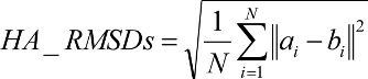
If the HA_RMSDs is "-1000.0", then there is an inconsistency in the number of heavy atoms between the reference and the docked conformer.
(2) Minimum-distance heavy-atom RMSD (HA_RMSDm): This measure is based on the RMSD implementation used in AutoDock Vina (Trott and Olson, J. Comput. Chem. 2010), which does not explicitly enforce one-to-one mapping. Rather, atom pairings between reference conformation a and pose conformation b are determined by the minimum distance to any atom of the same element type, and it may be an under-prediction of the true RMSD.
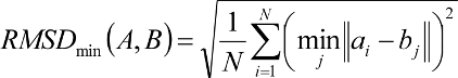

(3) Hungarian (symmetry-corrected) heavy-atom RMSD (HA_RMSDh):
The final RMSD implementation is based on an O(N^4) implementation of the Hungarian algorithm (Kuhn, Nav. Res. Logist. Q. 1955; Munkres, J. Soc. Indust. Appl. Math. 1957). The algorithm solves the optimal assignment between a set of reference ligand atoms a and a set of pose ligand atoms b of the same size. For all groups of atoms of the same Sybyl atom type, a cost matrix M is populated where each matrix element mij is equal to the distance-squared between reference atom ai and pose atom bj. The Hungarian algorithm is used to determine one-to-one assignments between reference and pose ligand atoms such that the total distance between atoms is minimized. The new assignments c(i) are fed into the standard RMSD function in order to compute a symmetry-corrected RMSD. If the HA_RMSDh is "-1000.0",
then there is an inconsistency in the number of atoms of at least one atom type between the reference and the docked conformer.
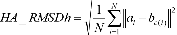
2.8.1 Ligand RMSD Parameters
| Parameter |
Description |
Default Value |
| calculate_rmsd |
Calculate root mean square deviation? |
no |
| use_rmsd_reference_mol |
Does the user want to use a reference molecule to calculate rmsd? |
no |
| rmsd_reference_filename |
The path to the rmsd reference molecule |
N/A |
RETURN TO TABLE OF CONTENTS
2.9.
Orienting the Ligand
2.9.1. Sphere
Matching
The rigid body orienting code is written as a
direct implementation of the isomorphous subgraph matching method of
Crippen and Kuhl (Kuhl
et al. J. Comput. Chem. 1984).
All receptor sphere pairs and atom center pairs are considered for
inclusion in a matching clique. This is more computationally demanding
than the clique matching algorithm implemented in previous versions
that used a distance binning algorithm to restrict the clique search,
in which pairs of spheres and atom centers were binned by distance.
Only sphere pairs and center pairs that were within the same distance
bin were considered as potential matches
(Ewing and Kuntz. J.
Comput. Chem. 1997).
The clique matching implementation avoids bin
boundaries that prevent some receptor sphere and ligand atom pairs from
matching, and, as a result, it can find good matches missed by previous
versions of DOCK. The rigid body rotation code has also been corrected
to avoid a singularity that occurred if the spheres in the match lay
within the same plane.
There are two types of ligand
orientation currently available:
(1) Automated Matching —Specify the
number of orientations, and DOCK will generate matches until enough
orientations passing the bump filter have been formed. Matches are
formed best first, with respect to the difference in the ligand and
site point internal distances.
(2) Manual Matching —Specify the distance and node
parameters,
and DOCK will generate all the matches which satisfy them. The number
of orientations scored is equal to the total matches minus the
orientations discarded by the user applied filters.
Multiple orientations may be
written out for each molecule using the write_orientations parameter,
otherwise only the best orientation is recorded.
Note that this feature is available only in serial DOCK;
in parallel DOCK only the best orientation is emitted.
In addition, now "VERBOSE ORIENTING STATS" are now printed when the verbose flag is used.
This prints orienting parameters, residual statistics, statistics on the nodes used in the match. See the Growth Tree And Statistics section below for an example of the output.
RETURN TO TABLE OF CONTENTS
2.9.2. Critical
Points
The critical_points feature is used
to focus the orientation search into a subsite of the receptor active
site (DesJarlais
et al. J. Comput-Aided Molec. Design. 1994
and Miller
et al. J. Comput. Aided Mol. Design. 1994).
For example, identifying molecules that interact with catalytic
residues might be of chief interest. Any number of points may be
identified as critical
(see Critical Points
in the sphgen documentation for information on labeling spheres),
and any number of groupings of these
points may be identified.
Cliques are checked for critical points by comparing spheres;
the criterion is that every grouping must have a coincident sphere
and the first coincident sphere found in a grouping terminates
further searching of that grouping.
An alternative to using critical points is to
discard all site points that are some distance away from the subsite of
interest, while retaining enough site points to define unique ligand
orientations. This feature can be highly effective at reducing matching
by five-fold or more. It is particularly useful to also assign chemical
labels to the critical points to further focus sampling.
In this case cliques are checked first for satisfaction of the
critical points criterion and then for satisfaction of the
chemical matching criteria.
RETURN TO TABLE OF CONTENTS
2.9.3. Chemical
Matching
The chemical_matching feature is used to
incorporate information about the chemical complementarity of a ligand
orientation into the matching process. In this feature, chemical labels
are assigned to site points
(see Chemical Matching
in the sphgen documentation for information on labeling spheres)
and ligand atoms (see Ligand File Input)
(Kuhl
et al. J. Comput. Chem. 1984).
The site point labels are based on the local receptor environment. The
ligand atom labels are based on user-adjustable chemical functionality
rules. These labeling rules are identified with the chemical_defn_file
parameter and reside in an editable file (see chem.defn).
A node in a match will produce an unfavorable interaction if the atom
and site point components have labels which violate a chemical match
rule. The chemical matching rules are identified with the
chemical_match_file parameter and reside in an editable file (see chem_match.tbl).
If a match will produce unfavorable interactions, then the match is
discarded. The speed-up from this technique depends how extensively
site points have been labeled and the stringency of the match rules,
but an improvement of two-fold or more can be expected.
RETURN
TO TABLE OF CONTENTS
2.9.4.
Macromolecular Docking
This feature has not been used in a long time.
Although DOCK is typically applied to small
ligand molecules, it can be used to study macromolecular ligands,
for example protein-protein and protein-DNA complexes.
The chief difference in protocol is that to use the
match_receptor_sites procedure for the orientation search, special
ligand centers must be used to represent the ligand. This is signaled
by setting the ligand_centers parameter. The ligand centers may be
constructed by sphgen and
must reside in a file identified with the ligand_center_file parameter.
See Shoichet et al. J.
Mol. Biol. 1991 for examples and discussion of
macromolecular docking.
RETURN TO TABLE OF CONTENTS
2.9.5 Orienting Parameters
| Parameter |
Description |
Default Value |
| orient_ligand |
Does the user want to orient the ligand to spheres? |
yes |
| automated_matching |
Does the user want to perform automated matching instead of manual matching? |
yes |
| distance_tolerance |
The tolerance in angstroms within which a pair of spheres is considered equivalent to a pair of centers (only turned on if manual matching is used) |
0.25 |
| distance_minimum |
The shortest distance allowed between 2 spheres - any sphere pair with a shorter distance is disregarded (only turned on with manually matching is used) |
0.0 |
| nodes_minimum |
The minimum number of nodes in a clique |
3 |
| nodes_maximum |
The maximum number of nodes in a clique |
10 |
| receptor_site_file |
The path to the file containing the receptor spheres |
receptor.sph |
| max_orientations |
The maximum number of orientations that will be cycled through |
1000 |
| critical_points |
Does the user want to use critical point sphere labeling to target orientations to particular spheres? |
no |
| chemical_matching |
Does the user want to use chemical coloring of spheres to match chemical labels on ligand atoms? |
no |
| chem_match_tbl |
The path to the file defining the legal chemical type matches/pairings (only turned on when chemical matching is used) |
chem_match.tbl |
| use_ligand_spheres |
Does the user want to use a sphere file representing ligand heavy atoms to orient the ligand? (typically used for macromolecular docking) |
no |
| ligand_sphere_file |
The path to the file containing the ligand sphere files (only turned on when use ligand spheres is used) |
ligand.sph |
RETURN TO TABLE OF CONTENTS
2.10.
Internal Energy Calculation
During growth and minimization, an internal energy scoring function can be used. The goal of the internal energy function is to reduce the occurrence of internal clashes during the torsional optimization. This function computes the repulsive Lennard-Jones term between all ligand atom pairs, excluding all 1-2, 1-3, and 1-4 pairs. (Currently, attractive Lennard-Jones and Coulombic terms are neglected; the aim is to eliminate internal clashes not to optimize the internal geometry. In addition, since there is no dihedral term in the force field, if the attractive terms are included the molecule might appear less physical.) The internal energy can be cut on or off; if cut on, it is reported in the output mol2 file and is used to prune conformers during growth. (This pruning is separate from the pruning that occurs based on interaction energy). We recommend the use of the internal energy function for all calculations.
2.9.5 Internal Energy Parameters
| Parameter |
Description |
Default Value |
| use_internal_energy |
Does the user want to use internal energy for growth and or minimization (only repulsive VDW) |
yes |
| internal_energy_rep_exp |
The VDW exponent only when use internal energy is turned on(DOCK is optimized for default value) |
12 |
| internal_energy_cutoff |
All conformers with an internal energy value above this cutoff are pruned(only turned on use internal energy is used) |
100.0 |
RETURN TO TABLE OF CONTENTS
2.11. Scoring
DOCK uses several types of scoring functions to
discriminate among orientations and molecules. Scoring is requested
using the score_molecules parameter. The scoring functions are
implemented with a hierarchical strategy. A master score class manages
all scoring functions that DOCK uses. Any of the DOCK scoring functions
can be selected as the primary, or used in combination with Descriptor Score.
The scoring function is used during rigid orienting,
anchor-and-grow steps, and minimization, which typically make many calls to the
scoring function.
RETURN TO TABLE OF CONTENTS
2.11.1. Bump Filter
Orientations and grow steps may be filtered prior
to scoring to discard those in which the molecule significantly overlaps receptor
atoms. This feature is enabled with the bump_filter flag. At the time
of construction of the bump filter, the amount of atom VDW overlap is
defined with the bump_overlap parameter (see Grid).
At the time of bump evaluation the number of allowed bumps is defined
with the max_bump_anchor and max_bump_growth parameter.
2.11.1 Bump Filter Parameters
| Parameter |
Description |
Default Value |
| bump_filter |
Does the user want to perform bump filter? |
no |
| bump_grid_prefix |
The prefix to the grid file containing the desired bump grid (only turned on when bump filter is used) |
grid |
| max_bumps_anchor |
The maximum allowed number of bumps for an anchor to pass the filter |
12 |
| max_bumps_growth |
The maximum allowed number of bumps for a molecule to pass the filter |
12 |
RETURN TO TABLE OF CONTENTS
2.11.2. Contact
Score
The contact score is a simple summation of the
number of heavy atom contacts between the ligand and receptor. At the
time of construction of the contact scoring grid, the distance
threshold defining a contact is set with the contact_cutoff_distance
(see Grid). Atom VDW overlaps
are penalized by
checking the bump filter grid, or with the contact_clash_overlap
parameter for the intramolecular score. The amount of penalty is
specified with the contact_clash_penalty parameter.
The contact score provides a
simple assessment
of shape complementarity. It can be useful for evaluating primarily
non-polar interactions.
2.11.2 Contact Score Parameters
| Parameter |
Description |
Default Value |
| contact_score_primary |
Does the user want to perform contact scoring as primary scoring function |
no |
| contact_score_cutoff_distance |
The distance threshold defining a contact when contact scoring is turned on |
4.5 |
| contact_score_clash_overlap |
Contact definition for use with intramolecular scoring when contact scoring is turned on |
0.75 |
| contact_score_clash_penalty |
The penalty for each contact overlap made when contact score is turned on |
50 |
| contact_score_grid_prefix |
The prefix to the grid files containing the desired contact when contact score is turned on |
grid |
Contact Score Output Components
- Contact_Score:
#sum of the number of heavy atom contacts between the ligand and receptor
RETURN TO TABLE OF CONTENTS
2.11.3. Grid-Based
Score
The grid-based score is based on the non-bonded terms of
the molecular mechanic force field (see Grid
for more background).
2.11.3.1 Grid Score Parameters
| Parameter |
Description |
Default Value |
| grid_score_primary |
Does the user want to perform grid-based energy scoring as the primary scoring function? |
yes |
| grid_score_rep_rad_scale |
Scalar multiplier of the radii for the repulsive portion of the VDW energy component only when grid score is turned on |
1.0 |
| grid_score_vdw_scale |
Scalar multiplier of the VDW energy component |
1 |
| grid_score_turn_off_vdw |
A flag to turn off vdw portion of scoring function when grid score vdw scale = 0 |
yes |
| grid_score_es_scale |
Flag to scale up or down the es portion of the scoring function when es scale is turned on |
1 |
| grid_lig_efficiency |
Flag to control use of ligand efficiency (Grid Score / # active heavy atoms) as primary score. |
no |
| grid_score_turn_off_es |
A flag to turn off es portion of scoring function when grid score es scale = 0 |
yes |
| grid_score_grid_prefix |
The prefix to the grid files containing the desired nrg/bmp grid |
grid |
When using Grid Score as a component scoring function in the Descriptor Score, the following parameters (questions asked in the DOCK input) may be needed.
2.11.3.1 Descriptor Grid Score Parameters
| Parameter |
Description |
Default Value |
| descriptor_grid_score_rep_rad_scale |
Scalar multiplier of the radii for the repulsive portion of the VDW energy component only when grid score is turned on |
1.0 |
| descriptor_grid_score_vdw_scale |
Scalar multiplier of the VDW energy component |
1 |
| descriptor_grid_score_turn_off_vdw |
A flag to turn off vdw portion of scoring function when grid score vdw scale = 0 |
yes |
| descriptor_grid_score_es_scale |
Flag to scale up or down the es portion of the scoring function when es scale is turned on |
1 |
| descriptor_grid_score_turn_off_es |
A flag to turn off es portion of scoring function when grid score es scale = 0 |
yes |
| descriptor_grid_score_grid_prefix |
The prefix to the grid files containing the desired nrg/bmp grid |
grid |
Grid Score Output Components
Note: output components will have the prefix desc_ if the scoring function is employed through Descriptor Score
- Grid_Score:
#sum of the van der Waals and electrostatic interactions
- Grid_vdw_energy:
#van der Waals interaction between the ligand and grid
- Grid_es_energy:
#electrostatic interaction between the ligand and grid
RETURN TO TABLE OF CONTENTS
2.11.4. DOCK3.5 Score
DOCK3.5 score is a variant of
Grid-based scoring (see Grid).
DOCK3.5 score calculates ligand desolvation in addition to
steric and electrostatic interactions between the ligand and receptor.
The electrostatic interactions between the ligand and the protein are
calculated from an electrostatic potential (ESP) map. The ESP map should
be calculated using finite difference Poisson-Boltzmann equation (PBE)
as implemented in the program DelPhi. We provide scripts for the
calculation; however,
DelPhi
is not distributed with DOCK; see also
here.
In DOCK 6.12, DOCK3.5 Score has been updated to match the DOCK 3.7 scoring function. We can convert electrostatic grids producted with Qnifft (Coleman, Plos One 2013). We can convert grids genereated with blastermaster.py to work with DOCK 6. SolvMap has also been updated to use solvent-excluded volume (MySinger, J Chem Inf Model 2010). solvent-excluded volume solvation grids are calculated with sevsol program.
In the DOCK scoring hierarchy DOCK3.5 Score follows GridScore.
2.11.4.1 DOCK 3.5 Score Parameters
| Parameter |
Description |
Default Value |
| dock3.5_score_primary |
Does the user want to perform dock3.5 scoring as the primary scoring function? |
no |
| dock3.5_vdw_score |
When dock3.5 scoring is turned on - calculate steric interaction from dock3.5 score |
yes |
| dock3.5_grd_prefix |
When dock3.5 scoring is turned on - path to files containing dock3.5 grids |
chem52 |
| dock3.5_electrostatic_score |
When dock3.5 scoring is turned on - calculate electrostatic interaction from ESP grid calculated using DelPhi |
yes |
| dock3.5_ligand_internal_energy |
Flag to add ligand internal energy to the scoring function |
no |
| dock3.5_ligand_desolvation_score |
Calculate total or volume based ligand desolvation from solvation grids |
volume |
| dock3.5_solvent_occlusion_file |
Occluded solvent grid of the receptor when desolvation score is turned on |
solvmap |
|
| dock3.5_redistribute_positive_desolvation |
Distribute positive partial atomic desolvation penalties when desolvation score is turned on |
no |
|
| dock3.5_write_atomic_energy_contrib |
Write contribution from each atom to total score |
no |
|
| dock3.5_score_vdw_scale |
Scalar multiplier of vdw energy component |
1.0 |
|
| dock3.5_score_es_scale |
Scalar multiplier of es energy component |
1.0 |
|
DOCK3.5 Score Output Components
- Chemgrid_Score:
#sum of the van der Waals and electrostatics interactions, plus other components (i.e. ligand and receptor desolvations) but depends on your input parameters
- Chemgrid_vdw_energy:
#van der Waals interaction between the ligand and receptor
- Chemgrid_es_energy:
#electrostatic interaction between the ligand and receptor
- Chemgrid_polsol:
#ligand polar desolvation component
- Chemgrid_apolsol:
#ligand apolar desolvation component
2.11.5.
Continuous Score
Continuous scoring may be used to evaluate a
ligand:receptor complex without the investment of a grid calculation,
or to perform a more detailed calculation without the numerical
approximation of the grid. See
Meng et al. J.
Comp. Chem. 1992.
When continuous scoring is requested, then
score parameters normally supplied to Grid,
must also be supplied to
DOCK. It is left to the user to make sure consistent values are
supplied to both programs.
The distance dependence of the Lennard-Jones
function is set with the cont_score_att_exp and cont_score_rep_exp
parameters. Typically a 6-12 potential is used, but it can be softened
up by using a 6-8 or 6-9 potential.
The source of the radii and well-depths is the same as for other
atom typing applications; see vdw.defn.
The distance dependence of the Coulombic function is set with the
cont_score_use_dist_dep_dielectric parameter.
The dielectric constant is adjusted with
the cont_score_dielectric parameter.
Note the correspondence of these parameters to those for
Grid Energy Scoring.
2.11.5.1 Continuous Score Parameters
| Parameter |
Description |
Default Value |
| continuous_score_primary |
Does the user want to perform continuous non-grid scoring as the primary scoring function? |
no |
| cont_score_rec_filename |
File that contains receptor coordinates |
receptor.mol2 |
| cont_score_att_exp |
VDW Lennard-Jones potential attractive exponent |
6 |
| cont_score_rep_exp |
VDW Lennard-Jones potential repulsive exponent |
12 |
| cont_score_rep_rad_scale |
Scalar multiplier of the radii for the repulsive portion of the vdw energy component only |
1.0 |
| cont_score_use_dist_dep_dielectric |
Distance dependent dielectric switch |
yes |
| cont_score_dielectric |
Dielectric constant for the electrostatic term |
|
|
| cont_score_vdw_scale |
Scalar multiplier of vdw energy component |
1 |
|
| cont_score_vdw_scale |
Flag to turn off vdw portion of the scoring function when cont_score_vdw_scale=0 |
yes |
|
| cont_score_es_scale |
Scalar multiplier of electrostatic energy component |
1.0 |
|
| cont_score_turn_off_es |
Flag to turn off es portion of the scoring function when cont_score_es_scale = 0 |
yes |
|
When using Continuous Score as a component scoring function in the Descriptor Score, the following parameters (questions asked in the DOCK input) may be needed.
2.11.5.2 Descriptor Continuous Score Parameters
| Parameter |
Description |
Default Value |
| descriptor_cont_score_rec_filename |
File that contains receptor coordinates |
receptor.mol2 |
| descriptor_cont_att_exp |
VDW Lennard-Jones potential attractive exponent |
6 |
| descriptor_cont_score_rep_exp |
VDW Lennard-Jones potential repulsive exponent |
12 |
| descriptor_cont_score_rep_rad_scale |
Scala multiplier of the radii for the repulsive portion of the VDW energy component only |
1.0 |
| descriptor_cont_score_use_dist_dep_dielectric |
Distance dependent dielectric switch |
yes |
| descriptor_cont_score_dielectric |
Dielectric constant for electrostatic term |
|
| descriptor_cont_score_vdw_scale |
Scalar multiplier of vdw energy component |
1 |
| descriptor_cont_score_turn_off_vdw |
Flag to turn off vdw portion of scoring function when descriptor_cont_score_vdw_scale = 0 |
yes |
|
| descriptor_cont_score_es_scale |
Scalar multiplier of es energy component |
1 |
|
| descriptor_cont_score_turn_off_es_scale |
Flag tot turn off es portion of scoring function when descriptor_cont_score_es_scale=0 |
yes |
|
Continuous Score Output Components
Note: output components will have the prefix desc_ if the scoring function is employed through Descriptor Score
- Continuous_Score
#sum of the van der Waals and electrostatic interactions
- Continuous_vdw_energy
#van der Waals interaction between the ligand and receptor
- Continuous_es_energy
#electrostatic interaction between the ligand and receptor
RETURN TO TABLE OF CONTENTS
2.11.6. Zou GB/SA Score
The Zou GB/SA scoring function is
a fast algorithm, the pairwise free energy model, for ligand binding
affinity calculations. Specifically, a pairwise descreening approximation
(Hawkins et al. Chem. Phys. Lett. 1995)
is used in calculations of the electrostatic energy contribution. The
algorithm also includes a procedure to account for the low dielectric
region that might form between the ligand and the receptor during
docking processes. It has been tested to obtain similar results
compared with the grid-based free energy model but with much less
computation efforts.
For more information on the scoring
function and specifics of the implementation, see
Liu et al. J. Phys. Chem. B. 2004.
Use of the DOCK -v verbose flag will produce more detailed energy breakdowns
than described below under Zou GB/SA Score Output Components.
2.11.6.1 Zou GB/SA Score Parameters
| Parameter |
Description |
Default Value |
| gbsa_zou_score_primary |
Flag to perform Zou GB/SA scoring as the primary scoring function |
no |
| gbsa_zou_gb_grid_prefix |
The path to the pairwise GB grids |
gb_grid |
| gbsa_zou_sa_grid_prefix |
The path to the SA grids |
sa_grid |
| gbsa_zou_vdw_grid_prefix |
The path to the nrg grids, used for the vdw portion of the GB/SA calculation |
grid |
| gbsa_zou_screen_file |
GB parameter file for electrostatic screening. Its located in the parameter dir by default |
screen.in |
| gbsa_zou_solvent_dielectric |
The value for the solvent dielectric |
78.300003 |
Zou GB/SA Score Output Components
- Zou_GBSA_Score:
#sum of the van der Waals, generalized born, solvent accessible surface area, and delta SA upon binding components
- Zou_GBSA_vdw_energy:
#van der Waals interaction between the ligand and receptor
- Zou_GBSA_gb_energy:
#generalized-born component
- Zou_GBSA_sa_energy:
#solvent accessible surface area
- Zou_GBSA_delta_SAS_hp_energy:
#change in the hydrophobic and total solvent accessible surface area upon ligand binding
RETURN TO TABLE OF CONTENTS
2.11.7.
Hawkins GB/SA Score
The Hawkins GB/SA score is an
implementation of the Molecular Mechanics Generalized Born Surface Area
(MM-GBSA) method originally described by (Srinivasan et al. J.
Am. Chem. Soc. 1998) and reviewed by (Kollman et al. Acc.
Chem. Res. 2000). This particular implementation of
MM-GBSA uses the pairwise GB solvation model reported by Hawkins,
Cramer and Truhlar (Hawkins
et al. Chem. Phys. Lett. 1995 , Hawkins et al. J.
Phys. Chem. 1996) with parameters described by
Tsui and Case (Tsui, et
al. Biopolymers 2001).
Solvent Accessible Surface Areas (SA) are computed using a C++
implementation of the Amber8 "icosahedra" algorithm.
The total
interaction between the ligand and receptor are represented by unscaled
Coulombic and Lennard jones energy terms (MM) plus the change (delta)
in solvation (GBSA) where deltaGBSA = GBSA
complex - (GBSA receptor + GBSA ligand). For any given
species GBSA = Gpolar ( GB energy) + Gnonpolar (SA*0.00542 +
0.92).
Note that if inner and outer dielectric constants are set to 1
(gas-phase) and 80 (water-phase), then GBSA terms are
formally equivalent to free energies of hydration that can be directly
compared with experimental data and useful for evaluating the accuracy
of different partial charge models (Rizzo et al. J.
Chem. Theory. Comput. 2006).
The Hawkins GB/SA score was intended to
be used for "single-point" calculations and the current implementation
is quite slow if energy minimization is performed at the same time.
However, an energy minimization is highly recommended prior to GBSA
single-point calculations given that scores can be very sensitive to
receptor-ligand geometry. Use of the -v flag will yield separate GBSA
terms for each species (complex, receptor, and ligand) and also include
raw icosahedra SA values in units of angstroms squared. This scoring
method requires that the vdw_AMBER_parm99.defn file be specified which
contains GB radii and scale parameters for each atom type.
2.11.7.1 Hawkins GB/SA Score Parameters
| Parameter |
Description |
Default Value |
| gbsa_hawkins_score_primary |
Flag to perform Hawkins GB/SA scoring as the primary scoring function |
no |
| gbsa_hawkins_score_rec_filename |
File that contains receptor coordinates |
receptor.mol2 |
| gbsa_hawkins_score_solvent_dielectric |
Dielectric constant for solvent |
78.5 |
| gbsa_hawkins_use_salt_screen |
use salt screening |
no |
| gbsa_hawkins_score_salt_conc(M) |
When salt screen is turned on, salt concentration for solvent at molar concentration |
0.0 |
| gbsa_hawkins_score_gb_offset |
GB radius offset |
0.09 |
| gbsa_hawkins_score_cont_vdw_and_es |
Flag to determine whether vdw and es values will be calculated continuously or from a grid |
yes |
| gbsa_hawkins_score_vdw_att_exp |
VDW Lennard-Jones potential attractive exponent |
6 |
| gbsa_hawkins_score_vdw_rep_exp |
VDW Lennard-Jones potential repulsive exponent |
12 |
| grid_score_rep_rad_scale |
Scalar multiplier for the radii for the repulsive portion of the vdw energy component only, not specific to gbsa_hawkins_score |
1.0 |
| gbsa_hawkins_score_grid_prefix |
The prefix of the grid file containing the vdw values when gbsa_hawkins_score_grid_cont_vdw_and_es = no |
grid |
Hawkins GB/SA Score Output Components
- Hawkins_GBSA_Score:
#sum of the van der Waals, electrostatics, generalized-born, solvent accessible surface area components
- Hawkins_GBSA_vdw_energy:
#van der Waals interaction between the ligand and receptor
- Hawkins_GBSA_es_energy:
#electrostatic interaction between the ligand and receptor
- Hawkins_GBSA_gb_energy:
#generalized-born component
- Hawkins_GBSA_sa_energy:
#solvent accessible surface area
RETURN TO TABLE OF CONTENTS
2.11.8. AMBER Score
The AMBER score provides a suite of functionality including:
AMBER molecular mechanics, implicit solvation,
and molecular dynamics simulation, receptor flexibility, and
conjugate gradient minimization.
The main disadvantages are more complicated input preparation
and increased computational expense.
2.11.8.1. AMBER Score Binding Energy
AMBER score implements molecular mechanics
implicit solvent simulations with the traditional all-atom
AMBER force field
(Pearlman et al.
Comp. Phys. Commun. 1995)
for protein atoms and the general AMBER force field (GAFF,
Wang et al.
J. Comp. Chem. 2004)
for ligand atoms. The interaction between the ligand and the receptor
is represented by electrostatic and van der Waals energy terms, and the
solvation energy is calculated using a Generalized Born (GB) solvation
model. The user has the option to choose one of the following GB models:
(i) Hawkins, Cramer and Truhlar pairwise GB model with parameters
described by Tsui and Case (gb=1) (
Tsui et al. Biopolymers 2001),
(ii) Onufriev, Bashford and Case model, GB(OBC) (gb=2)
( Onufriev et al.
Proteins 2004), and
(iii) a modified GB(OBC) (gb=5)
( Onufriev et al. Proteins
2004).
The surface area term is derived using a fast LCPO algorithm
( Weiser et al. J. Comp Chem 1999).
The AMBER score is calculated as:
E(Complex) - [ E(Receptor) + E(Ligand) ],
where E(Complex), E(Receptor), and E(Ligand) are, respectively, the
internal energies
of the complex, receptor, and ligand (all solvated) as approximated by
the AMBER force field
with a GB/SA solvation term as referenced above.
The calculation of each of these three energies uses the same protocol:
minimization with a conjugate gradient method
is followed by MD simulation (Langevin molecular dynamics at
constant temperature), another minimization, and a final energy
evaluation. The user can specify the number of
pre-MD-minimization cycles, the number of MD simulation steps,
and the number of post-MD-minimization cycles in the dock input file.
During the final energy evaluation, a surface area term is included.
The receptor energy is determined once.
The AMBER score energy protocol is performed for every ligand and
its corresponding complex.
The protocol that is performed with all default input parameters
was developed in the work of
Graves et al., 2008.
2.11.8.2. AMBER Score Receptor Flexibility
AMBER score enables all or a part of
the receptor to be flexible, in order
to reproduce the so-called "induced-fit".
The Cartesian coordinates of atoms that are flexible can be altered
during the AMBER score energy protocol.
The Cartesian coordinates of atoms that are not flexible cannot be altered
during the AMBER score energy protocol.
The flexible parts of the receptor-ligand complex
are specified with a movable region Dock input file parameter.
The movable region options are
ligand, everything, nothing, distance, and NAB atom expression.
For the ligand option, only the ligand is allowed to move
during minimization and MD simulation. For the everything option,
all the atoms in the receptor and the ligand are allowed to move.
No minimization or MD simulation occurs for the nothing option.
This is the only movable region option for which the ligand is
not flexible during the AMBER score energy protocol.
Consequently, close contacts can produce very large energies
because the AMBER force field can be sensitive to the
receptor-ligand geometry.
However, the nothing option is the fastest type of AMBER scoring.
The distance movable region option
selects residues that are allowed to move by receptor-ligand distance.
If any atom in a receptor residue is within
amber_score_movable_distance_cutoff angstroms
of the ligand then the whole residue is selected.
The ligand is represented by the active site sphere list, and thus
the movable receptor residues are well defined and
independent of any particular ligand molecule.
The ligand is always movable.
The selected residues are emitted with the -v verbose flag as
a NAB atom expression.
The NAB atom expression movable region option is
based on the program
Nucleic Acid Builder (NAB).
Every atom in a NAB molecule has a unique name. This name is
composed of the strand name, the residue number and the atom name.
A NAB atom expression is a character string that contains one or more patterns
that match a set of atom names in a molecule.
The two Dock input file parameters associated with this option specify
the sets of atoms in the receptor and in the complex that are movable.
To date our use of of this option has always specified that the
set of complex movable atoms is the set of receptor movable atoms plus
all atoms of the ligand;
however, the two input parameters allow disparate usage.
In DOCK a strand name is in fact a strand sequence number, and
in a receptor-ligand complex, the ligand is always first in the
sequence. Thus, a receptor molecule with two strands has strand
names of "1" and "2"; in a corresponding receptor-ligand complex,
the ligand (which is almost certainly single stranded) has strand
name "1" and the receptor has strand names of "2" and "3".
NAB atom expressions contain three subexpressions separated by colons.
They represent the strand, residue and atom parts of the atom expression.
Not all three parts are required. An empty part selects all strands,
residues or atoms depending on which parts are empty.
Each subexpression consists of a comma separated list of patterns,
or for the residue part, patterns and/or number ranges.
Several atom expressions may be placed
in a single character string by separating them with the vertical bar.
Patterns in atom expressions are similar to Unix shell expressions. Each
pattern is a sequence of one or more single character patterns and/or stars.
The star matches zero or more occurrences of any single character.
Each part of an atom expression is composed of a comma separated list of
limited regular expressions, or in the case of the residue part, limited
regular expressions and/or ranges. A range is a number or a
pair of numbers separated by a dash.
The
NAB
manual contains more information on atom expressions.
Here are some examples of NAB atom expressions:
- :SER:
#Select all atoms in any residue named SER. All three parts are
present but both the strand and atom parts are empty. The atom
expression :SER selects the same set of atoms.
- ::C,CA,N,O
#Select all atoms with names C, CA, N or O in all residues in all strands
(typically the peptide backbone).
- 1:1-10,13:CA,C,N
#Select all atoms named CA,C,N in residues 1-10 and 13 in strand 1.
- ::C*[^1]
#The [^1] is an example of a negated
character class. It matches any character in the last position except 1.
In this case, it will match all the atoms starting with C, such as CA, CB, CG2, but not those ending with 1, such as CD1, CE1.
- 2::|1:50,100:O*,N*
#Select all atoms in strand 2. Select all atoms whose name starts
with O and N in residue 50, 100 in strand 1.
Note that the vertical bar separates the two strands
- 4::|2::|1::
#Select strand 4, 2 and 1.
- :: or :
#Select all atoms in the molecule.
2.11.8.3. AMBER Score Inputs
AMBER score requires many additional input files beyond those of
other DOCK scoring functions.
All the input files, such as the prmtop, frcmod, amber.pdb, etc.
should be generated prior to running the DOCK AMBER score.
Two perl scripts, prepare_amber.pl and prepare_rna_amber.pl, have
been provided for this purpose.
The script prepare_rna_amber.pl differs from prepare_amber.pl
in that the former treats all nucleic acids as RNA
whereas the latter treats them as DNA; in addition,
prepare_rna_amber.pl supports the RNA specific features
to neutralize to a total charge of zero
and to solvate with water.
The usage of these is, e.g.,
prepare_amber.pl ligand_mol2_file receptor_PDB_file
For example, if lig.mol2 is the name of the file that contains the ligand
in mol2 format and rec.pdb is the name of the file that contains the
receptor in PDB format then enter: prepare_amber.pl lig.mol2 rec.pdb
These scripts can process a mol2 file containing multiple ligands
(usually the output from a previous DOCK run).
See the section
Amber Score Preparation Scripts
and the
tutorials
for more information on how
to use these scripts to generate the input files.
The prepare amber perl scripts call
other scripts and programs, such as antechamber
to calculate the AM1-BCC charges for the ligands, and
tLEaP
to assign the parm94 parameter set for protein
atoms and the GAFF parameter set for ligand atoms.
A metal ions library (parameters/leap/cmd/leaprc.dock.ions),
a cofactor library (parameters/leap/cmd/leaprc.dock.cofactors),
and a hook for a user library (parameters/leap/cmd/leaprc.dock.user),
are automatically processed by tleap.
The latter library provides an override mechanism for the global
handling of common problems such as missing force field parameters.
Detection of parmchk "ATTN, needs revision" messages for missing force
field parameters and a local recovery mechanism for the frcmod files
exists. The recovery process is described in the warning message
and involves creating a file with the extension ".frcmod.revised file".
With knowledge of and experience using
AMBER
one could create the input files manually; see the amberize scripts
for the gory details. Note that the ligand_atom_file, which has
the extension ".amber_score.mol2", must have a TRIPOS
AMBER_SCORE_ID
section for every ligand.
2.11.8.4. AMBER Score Outputs
The AMBER score output in the DOCK output contains energy
terms for each species (complex, receptor, and ligand) such that
the sum of the terms is equal to the score;
in particular, note that the receptor and ligand values have been negated.
Use of the DOCK -v verbose flag will produce detailed energy breakdowns;
the formats and definitions of this information are discussed in the
the NAB manual:
Nucleic Acid Builder (NAB).
The verbose output is best captured via UNIX shell file redirection
as opposed to the DOCK -o flag.
The AMBER score output in the ligand_outfile_prefix_scored.mol2 file
contains the ligand coordinates extracted from the final structure
of the complex (i.e., the structure after the
AMBER score energy protocol is performed).
The ligand charges are from the ligand prmtop file.
The ligand atom types are the normal ones from DOCK and are not the GAFF
atom types used by AMBER score.
The AMBER score uses the following method for emitting all
the final structures in their entirety.
The AMBER score will create a file with the extension
".final_pose.amber.pdb" for every species (receptor, ligands, and complexes)
that contains any movable region (regardless of whether that region
actually exists or actually does move).
Thus, for the distance, everything, and NAB atom expression options
of the movable region, a file for the receptor
(amber_score_receptor_file_prefix.final_pose.amber.pdb) and two for each
ligand,complex pair
(AMBER_SCORE_ID.final_pose.amber.pdb,
amber_score_receptor_file_prefix.AMBER_SCORE_ID.final_pose.amber.pdb)
will be created; for the nothing option of the movable region,
no files will be created.
In addition, if the -v verbose flag is present then the AMBER score will
create an AMBER restart file with the extension ".final_pose.amber.restart"
for every species (receptor, ligands, and complexes)
that contains any movable region (regardless of whether that region
actually exists or actually does move).
2.11.8.5. AMBER Score in Practice
Here is some general advice on the AMBER score.
Since it is slower and more complicated than the other scoring functions,
one should proceed carefully when using the AMBER score as the sole
primary score.
The most obvious use is to rescore, with the default amber_score
input parameters, the ligands
that have been already scored using one of the faster scoring functions.
In fact, due to current software constraints it is not possible to use
AMBER score as the primary score when orient_ligand=yes.
In general, the input preparation for AMBER score is more involved than for
the other scores. Effectively, one needs to generate input files for
AMBER.
In particular,
examine the amberize*.out and *.log files for warnings and errors.
(Note that the environment variable AMBERHOME should Not be defined
when using AMBER score.)
Experience using AMBER will help in understanding and judging
the impact of the messages in these files. Correcting problems may
involve substantial effort. This
DOCK-Fans post
discusses in detail the recovery options for failing ligands.
2.11.8.6 AMBER Score Parameters
| Parameter |
Description |
Default Value |
| amber_score_primary |
Flag to perform amber scoring as the primary scoring function |
no |
| amber_receptor_file_prefix |
Prefix of the file that contains receptor coordinates that was used in the prepare_amber.pl input files preparation step. |
rec |
| amber_score_movable region |
The region that will be flexible during the scoring protocol.(Options: distance, everything, ligand, nab_atom_expression, nothing) |
ligand |
| receptor_site_file |
The file containing the receptor spheres that define the active site. This is not specific to amber score. This is active for amber_score_movable_region=distance. |
receptor.sph |
| amber_score_receptor_movable_atom_expr |
NAB atom expression defining the movable receptor region. This is active only for amber_score_movable_region=nab_atom_expression |
|
| amber_score_complex_movable_atom_expr |
NAB atom expression defining the movable complex region. This is active only for amber_score_movable_region=nab_atom_expression |
|
| amber_score_minimization_rmsgrad |
Minimization convergence criterion for the root-mean-square of the components of the gradient. |
0.01 |
| amber_score_before_md_minimization_cycles |
Number of conjugate gradient minimization cycles to be performed before MD. |
100 |
| amber_score_md_steps |
Number of Molecular Dynamics (MD) steps to be performed. |
3000 |
| amber_score_after_md_minimization_cycles |
Number of conjugate gradient minimization cycles to be performed after MD. |
100 |
| amber_score_gb_model |
GB model to be used |
5 |
| amber_score_nonbonded_cutoff |
Non-bonded cutoff in angstroms for the energy calculation. |
18.0 |
| amber_score_temperature |
Temperature at which MD should be performed. |
300 |
| amber_score_abort_on_unprepped_ligand |
Control over the behavior for an unprepped ligand. |
yes |
AMBER Score Output Components
- Amber_Score:
#sum of the complex, receptor, and ligand energies
- Amber_complex_energy:
#energy component of the complex
- Amber_receptor_energy:
#energy component of the receptor
- Amber_ligand_energy:
#energy component of the ligand
RETURN TO TABLE OF CONTENTS
2.11.9. Footprint Score
The Footprint score (previously named Descriptor score in DOCK6.7) is a scoring function that calculates
intermolecular hydrogen bonds, and footprint comparisons, in addition to standard intermolecular
energies (VDW and ES). Descriptor score is now the name of a new function that allows for combinations
of many different scoring functions to be used (see discussion below).
Intermolecular Energy
Intermolecular Energies (VDW, ES) are calculated the same way as in Continuous Score.
Hydrogen Bonds
A geometric definition of Hydrogen bonds is employed.
We define 3 atoms XD, HD, and XA as the heavy atom donor,
donated hydrogen, and heavy atom acceptor, respectively. There is a hydrogen bond present if the following two conditions are met:
(1) The distance between HD and XA is less than or equal to 2.5 angstroms;
(2) The angle defined by XD, HD, and XA is between 120 and 180 degrees.
Footprints
Footprints are a per-residue decomposition of interactions between the ligand and
the receptor. This can be performed for all three terms VDW, ES, HB.
See Balius et al. The method was validated using a testset of 780 structures. See Mukherjee et al.
Footprints Similarity
Two footprints can be compared in three ways:
Standard Euclidean, Normalized Euclidean, Pearson Correlation.
Footprints are used to gauge how similar two poses or two molecules are to one-another. For applications to virtual screening applications a reference is required.
There are to choices for a reference:
(1) One can give a mol2 file containing a reference molecule, and footprints will be calculated.
(2) One can pass a text file containing VDW, ES, and H-bond footprints.
The following is an example of format for the footprint reference text file:
####################################
###  Reference FP
####################################

 resname   resid     vdw_ref      es_ref  hb_ref
    GLY1       1   -0.000045   -0.000061       0
    GLU2       2   -0.000226    0.000032       0
    ALA3       3   -0.000174   -0.000093       0
    PRO4       4   -0.000266    0.000186       0
    ASN5       5   -0.001091    0.000538       0
    GLN6       6   -0.000612    0.000165       0
    ALA7       7   -0.001325   -0.000591       0
    LEU8       8   -0.002368    0.000552       0
    LEU9       9   -0.007224    0.000388       0
   ARG10      10   -0.007143   -0.008906       0
   ILE11      11   -0.004132    0.000615       0
   LEU12      12   -0.012233   -0.000404       0
   LYS13      13   -0.002511   -0.003366       0
   GLU14      14   -0.004349    0.005031       0
   THR15      15   -0.001461    0.000304       0
Residue selections
There are different choices for selection of residues:
(1) All residues.
(2) Residues chosen using a threshold (union of the sets of reference and pose). The VDW, ES, and HB footprints may have different residues chosen in this case.
(3) Selected residues.
Note that for (2) and (3) the remaining residue interaction may be placed in a remainder value included in the footprint.
2.11.9.1 Footprint Score Parameters
| Parameter |
Description |
Default Value |
| footprint_similarity_score_primary |
Flag to perform footprint scoring as the primary scoring function |
no |
| fps_score_use_footprint_reference_mol2 |
Use a molecule to calculate footprint reference. |
no |
| fps_score_footprint_reference_mol2_filename |
Path to the reference mol2 file - only used when footprint reference mol2 is turned on. |
ligand_footprint.mol2 |
| fps_score_use_footprint_reference_txt |
Use a pre-calculated footprint reference in text format. |
no |
| fps_score_footprint_reference_txt_filename |
Path to the reference txt file - only used when footprint reference txt is turned on. |
ligand_footprint.txt |
| fps_score_foot_compare_type |
Footprint similarity calculation methods (Options: Euclidean, Pearson). If Pearson, the correlation coefficient as the metric to compare the footprints. When the value is 1 then there is perfect agreement between the two footprints. When the value is 0 then there is poor agreement between the two footprints. If Euclidean, the Euclidean distance as the metric to compare the footprints. When the value is 0 then there is perfect agreement between the two footprints. As the agreement gets worse between the two footprints the value increases. |
Euclidean |
| fps_score_normalize_foot |
normalization is used only with Euclidean distance. |
no |
| fps_score_foot_comp_all_residue |
If yes all residues are used for calculating the footprint. |
yes |
| fps_score_choose_foot_range_type |
User can use to determine the type of the range of the footprint by either specifying a residue range or defining a threshold. If specify_range, the user chooses to use a residue range and all footprints will be evaluated only on this residue range. First residue id = 1 not 0. If threshold, the user chose to use a residue range that is defined by only residues that have magnitudes that exceed the specified thresholds. (Options: specify_range, threshold) |
specify_range |
| fps_score_vdw_threshold |
Specify threshold for van der Waals energy, when threshold is turned on. |
1 |
| fps_score_es_threshold |
Specify threshold for electrostatic energy, when threshold is turned on. |
1 |
| fps_score_hb_threshold |
specify threshold for hydrogen bonds (integers). 0.5 means that all none zeros are used, when threshold is turned on. |
0.5 |
| fps_score_use_remainder |
Interaction remainder is all remaining residues not included individually |
yes |
| fps_score_rec_filename |
File that contains receptor coordinates |
receptor.mol2 |
| fps_score_att_exp |
VDW Lennard-Jones potential attractive exponent |
6 |
| fps_score_rep_exp |
VDW Lennard-Jones potential repulsive exponent |
12 |
| fps_score_rep_rad_scale |
Scalar multiplier of the radii for the repulsive portion of the VDW energy component ONLY |
1 |
| fps_score_use_distance_dependent_dielectric |
Distance dependent dielectric switch |
yes |
| fps_score_dielectric |
Dielectric constant for electrostatic term |
4.0 |
| fps_score_vdw_scale |
Scalar multiplier of vdw energy component |
1 |
| fps_score_es_scale |
Scalar multiplier of es energy component |
1 |
| fps_score_hb_scale |
Scalar multiplier of hb energy component |
0 |
| fps_score_internal_scale |
Scalar multiplier of internal energy component |
0 |
| fps_score_fp_vwd_scale |
Scalar multiplier of vdw footprint component |
0 |
| fps_score_fp_es_scale |
Scalar multiplier of es footprint component |
0 |
| fps_score_fp_hb_scale |
Scalar multiplier of hb footprint component |
0 |
When using Footprint Score as a component scoring function in the Descriptor Score, the following parameters (questions asked in the DOCK input) may be needed.
2.11.9.2 Descriptor Footprint Score Parameters
| Parameter |
Description |
Default Value |
| descriptor_fps_score_use_footprint_reference_mol2 |
Use a molecule to calculate footprint reference. |
no |
| descriptor_fps_score_footprint_reference_mol2_filename |
Path to the reference mol2 file - only used when footprint reference mol2 is turned on. |
ligand_footprint.mol2 |
| descriptor_fps_score_use_footprint_reference_txt |
Use a pre-calculated footprint reference in text format. |
no |
| descriptor_fps_score_footprint_reference_txt_filename |
Path to the reference txt file - only used when footprint reference txt is turned on. |
ligand_footprint.txt |
| descriptor_fps_score_foot_compare_type |
Footprint similarity calculation methods (Options: Euclidean, Pearson). If Pearson, the correlation coefficient as the metric to compare the footprints. When the value is 1 then there is perfect agreement between the two footprints. When the value is 0 then there is poor agreement between the two footprints. If Euclidean, the Euclidean distance as the metric to compare the footprints. When the value is 0 then there is perfect agreement between the two footprints. As the agreement gets worse between the two footprints the value increases. |
Euclidean |
| descriptor_fps_score_normalize_foot |
normalization is used only with Euclidean distance. |
no |
| descriptor_fps_score_foot_comp_all_residue |
If yes all residues are used for calculating the footprint. |
yes |
| descriptor_fps_score_choose_foot_range_type |
User can use to determine the type of the range of the footprint by either specifying a residue range or defining a threshold. If specify_range, the user chooses to use a residue range and all footprints will be evaluated only on this residue range. First residue id = 1 not 0. If threshold, the user chose to use a residue range that is defined by only residues that have magnitudes that exceed the specified thresholds. (Options: specify_range, threshold) |
specify_range |
| descriptor_fps_score_vdw_threshold |
Specify threshold for van der Waals energy, when threshold is turned on. |
1 |
| descriptor_fps_score_es_threshold |
Specify threshold for electrostatic energy, when threshold is turned on. |
1 |
| descriptor_fps_score_hb_threshold |
specify threshold for hydrogen bonds (integers). 0.5 means that all none zeros are used, when threshold is turned on. |
0.5 |
| descriptor_fps_score_use_remainder |
Interaction remainder is all remaining residues not included individually |
yes |
| descriptor_fps_score_rec_filename |
File that contains receptor coordinates |
receptor.mol2 |
| descriptor_fps_score_att_exp |
VDW Lennard-Jones potential attractive exponent |
6 |
| descriptor_fps_score_rep_exp |
VDW Lennard-Jones potential repulsive exponent |
12 |
| descriptor_fps_score_rep_rad_scale |
Scalar multiplier of the radii for the repulsive portion of the VDW energy component ONLY |
1 |
| descriptor_fps_score_use_distance_dependent_dielectric |
Distance dependent dielectric switch |
yes |
| descriptor_fps_score_dielectric |
Dielectric constant for electrostatic term |
4.0 |
| descriptor_fps_score_vdw_scale |
Scalar multiplier of vdw energy component |
1 |
| descriptor_fps_score_es_scale |
Scalar multiplier of es energy component |
1 |
| descriptor_fps_score_hb_scale |
Scalar multiplier of hb energy component |
0 |
| descriptor_fps_score_internal_scale |
Scalar multiplier of internal energy component |
0 |
| descriptor_fps_score_fp_vwd_scale |
Scalar multiplier of vdw footprint component |
0 |
| descriptor_fps_score_fp_es_scale |
Scalar multiplier of es footprint component |
0 |
| descriptor_fps_score_fp_hb_scale |
Scalar multiplier of hb footprint component |
0 |
Footprint Similarity Score Output Components
Note: output components will have the prefix desc_ if the scoring function is employed through Descriptor Score
- Footprint_Similarity_Score:
#sum of the van der Waals, electrostatic, and hbond footprint similarity scores
- FPS_vdw_energy:
#van der Waals interaction between the ligand and receptor
- FPS_es_energy:
#electrostatic interaction between the ligand and receptor
- FPS_num_hbond:
#number of hydrogen-bonds
- FPS_vdw+es_energy:
#sum of the van der Waals and electrostatic components
- FPS_vdw_fps:
#van der Waals footprint similarity score
- FPS_es_fps:
#electrostatic footprint similarity score
- FPS_hb_fps:
#hbond footprint similarity score
- FPS_vdw_fp_numres:
#number of residues in the receptor considered during the calculation
- FPS_es_fp_numres:
#number of residues in the receptor considered during the calculation
- FPS_hb_fp_numres:
#number of residues in the receptor considered during the calculation
RETURN TO TABLE OF CONTENTS
2.11.10. MultiGrid Score
The MultiGrid Score is similar to the Footprint Score described in the previous section, except that in the case of the Multi-Grid Score, the pair-wise interaction energies are computed over multiple grids rather than in Cartesian space.
This is done to improve the tractability of FPS calculations as well as to make it simple to combine FPS and standard Grid Score.
If the multiple grids are prepared as recommended than the sum of the interactions with each grid should equal the interaction of a standard DOCK grid representing the entire target.
By default MultiGrid score will equal the sum of the interactions with all grids plus a FPS component generated by treating each grid as a protein residue.
User defined scaling factors allow MultiGrid score to be set to equal Grid score, FPS score or any combination thereof.
Generally, "important" receptor residues are identified before-hand based on the magnitude of their interaction with the reference ligand, then a unique grid is generated to represent each of those residues.
Finally, a "remainder" grid is generated to represent all remaining receptor residues.
The scoring function itself will then calculate intermolecular VDW and ES energies for the reference ligand and pose ligand on each of the grids (also called footprints), then it will calculate the footprint similarity using either the Standard Euclidean, Normalized Euclidean, or Pearson Correlation similarity metrics as described above.
To aid in the selection of important residues and automate the creation of grids, a wrapper python script has been included called "multigrid_fp_gen.py".
Grid Generation
Here is an example script for generating the grids:
#############################################################################
dock6 -i important_residues.in -o important_residues.out
multigrid_fp_gen.py rec.mol2 resid grid.in `grep -A 1 range_union important_residues.out | sed -e'/range_union/d' -e'/--/d' -e's/ //g' | tr ',' '\n' | sort -nu`
#############################################################################
This script can be found in the test suite
(install/test/fp_multigrid_generation/getrange_mkgrids).
In this script dock is run using Footprint Score
to obtain the important residues, and then the dock output file is processed
with grep, sed, and sort to give the range in the format needed by the
python grid generation wrapper script.
Several files are needed including a box.pdb file and a grid input file to generate the grids, for example:
#############################################################################
compute_grids yes
grid_spacing 0.4
output_molecule yes
contact_score no
chemical_score no
energy_score yes
energy_cutoff_distance 999
atom_model a
attractive_exponent 6
repulsive_exponent 9
distance_dielectric yes
dielectric_factor 4
bump_filter yes
bump_overlap 0.75
receptor_file ./temp.mol2
box_file ./box.pdb
vdw_definition_file ../../../parameters/vdw_AMBER_parm99.defn
score_grid_prefix ./temp.rec
receptor_out_file ./temp.rec.grid.mol2
#############################################################################
This grid program produces the temp grid files which are then renamed by the python script.
2.11.10.1 MulitGrid FPS Score Parameters
| Parameter |
Description |
Default Value |
| multigrid_score_primary |
Flag to perform MultiGrid FPS scoring as the primary scoring function |
no |
| multigrid_score_rep_rad_scale |
Scale the VDW repulsive exponent only by this amount. |
1.0 |
| multigrid_score_vdw_scale |
Scale both VDW terms in the molecular mechanics interaction function by this amount. |
1.0 |
| multigrid_score_es_scale |
Scale both ES terms in the molecular mechanics interaction function by this amount. |
20 |
| multigrid_score_number_of_grids |
The number of grids to be used, which typically includes N selected grids plus one remainder grid. |
20 |
| multigrid_score_grid_prefix0 |
Provide prefixes to identify the grids. Note that the first grid starts at '0'. The last grid should be the remainder grid. This must be done for each grid. |
multigrid0 |
| multigrid_score_individual_rec_ensemble |
Flag for individual receptor (standard) or multiple receptor (not implemented yet). |
no |
| multigrid_score_weights_text |
Flag for providing a textfile as input for the reference footprint. |
no |
| multigrid_score_footprint_text |
Name of the reference footprint input text file, when multigrid_score_weight_text is turned on. |
reference.txt |
| multigrid_score_fp_ref_mol |
Flag for providing a MOL2 as input for the reference footprint. |
no |
| multigrid_score_footprint_ref |
Name of the reference footprint input MOL2 file, when multigrid_score_fp_ref_mol is turned on. |
reference.mol2 |
| multigrid_score_foot_compare_type |
Footprint similarity calculation methods (Options: Euclidean, Pearson). If Pearson, the correlation coefficient as the metric to compare the footprints. When the value is 1 then there is perfect agreement between the two footprints. When the value is 0 then there is poor agreement between the two footprints. If Euclidean, the Euclidean distance as the metric to compare the footprints. When the value is 0 then there is perfect agreement between the two footprints. As the agreement gets worse between the two footprints the value increases. |
Euclidean |
| multigrid_score_normalize_foot |
normalization is used only with Euclidean distance. |
no |
| multigrid_score_vdw_euc_scale |
Scaling factor for VDW term. when using euclidean |
1.0 |
| multigrid_score_es_euc_scale |
Scaling factor for ES term when using euclidean |
1.0 |
| multigrid_score_vdw_norm_scale |
Scaling factor for VDW term. euclidean and normalize |
10.0 |
| multigrid_score_es_norm_scale |
Scaling factor for ES term. Flags if using Pearson Correlation similarity metric for footprint comparison. |
10.0 |
| multigrid_score_vdw_cor_scale |
Scaling factor for VDW term |
-10.0 |
| multigrid_score_es_cor_scale |
Scaling factor for ES term |
-10.0 |
When using MultiGrid FPS Score as a component scoring function in the Descriptor Score, the following parameters (questions asked in the DOCK input) may be needed.
| Parameter |
Description |
Default Value |
| descriptor_multigrid_score_rep_rad_scale |
Scale the VDW repulsive exponent only by this amount. |
1.0 |
| descriptor_multigrid_score_vdw_scale |
Scale both VDW terms in the molecular mechanics interaction function by this amount. |
1.0 |
| descriptor_multigrid_score_es_scale |
The number of grids to be used, which typically includes N selected grids plus one remainder grid. |
20 |
| descriptor_multigrid_score_number_of_grids |
Path to the reference txt file - only used when footprint reference txt is turned on. |
ligand_footprint.txt |
| descriptor_multigrid_score_grid_prefix0 |
Provide prefixes to identify the grids. Note that the first grid starts at '0'. The last grid should be the remainder grid. This must be done for each grid. |
multigrid0 |
| descriptor_multigrid_score_individual_rec_ensemble |
Flag for individual receptor (standard) or multiple receptor (not implemented yet). |
no |
| descriptor_multigrid_score_weights_text |
Flag for providing a textfile as input for the reference footprint. |
no |
| descriptor_multigrid_score_footprint_text |
Name of the reference footprint input text file, when multigrid_score_weight_text is turned on. |
reference.txt |
| descriptor_multigrid_score_fp_ref_mol |
Flag for providing a MOL2 as input for the reference footprint. |
no |
| descriptor_multigrid_score_footprint_ref |
Name of the reference footprint input MOL2 file, when multigrid_score_fp_ref_mol is turned on. |
reference.mol2 |
| descriptor_multigrid_score_foot_compare_type |
Footprint similarity calculation methods (Options: Euclidean, Pearson). If Pearson, the correlation coefficient as the metric to compare the footprints. When the value is 1 then there is perfect agreement between the two footprints. When the value is 0 then there is poor agreement between the two footprints. If Euclidean, the Euclidean distance as the metric to compare the footprints. When the value is 0 then there is perfect agreement between the two footprints. As the agreement gets worse between the two footprints the value increases. |
Euclidean |
| descriptor_multigrid_score_normalize_foot |
normalization is used only with Euclidean distance. |
no |
| descriptor_multigrid_score_vdw_euc_scale |
Scaling factor for VDW term. when using euclidean |
1.0 |
| descriptor_multigrid_score_es_euc_scale |
Scaling factor for ES term when using euclidean |
1.0 |
| descriptor_multigrid_score_vdw_norm_scale |
Scaling factor for VDW term. euclidean and normalize |
10.0 |
| descriptor_multigrid_score_es_norm_scale |
Scaling factor for ES term. Flags if using Pearson Correlation similarity metric for footprint comparison. |
10.0 |
| descriptor_multigrid_score_vdw_cor_scale |
Scaling factor for VDW term |
-10.0 |
| descriptor_multigrid_score_es_cor_scale |
Scaling factor for ES term |
-10.0 |
MultiGrid Score Output Components
Note: output components will have the prefix desc_ if the scoring function is employed through Descriptor Score
- MultiGrid_Score:
#sum of the van der Waals, electrostatic energies, van der Waals, and electrostatic footprint similarity scores
- MGS_vdw_energy:
#van der Waals interaction between the ligand and grid
- MGS_es_energy:
#electrostatic interaction between the ligand and grid
- MGS_vdw+es_energy:
#sum of the van der Waals and electrostatic components
- MGS_vdw_fps:
#van der Waals footprint similarity score
- MGS_es_fps:
#electrostatic footprint similarity score
- MGS_vdw+es_fps:
#sum of the van der Waals and electrostatic footprint similarity scores
RETURN TO TABLE OF CONTENTS
2.11.11. Pharmacophore Matching Similarity Score
The Pharmacophore Matching Similarity score is a scoring function that calculates the level of pharmacophore overlap between a reference molecule and a candidate molecule in three dimensional space.
Pharmacophore Features
Pharmacophore features are derived from the pharmacophore type of atoms in the molecule defined by the SYBYL atom type and atom environment. Definitions of pharmacophore features used in this scoring function include: 1) hydrophobic (PHO), 2) hydrogen bond donor (HBD), 3) hydrogen bond acceptor (HBA), 4) aromatic ring (ARO), 5) nonaromatic ring (RNG), 6) positively charged (POS), and 7) negatively charged (NEG) features. See Jiang et al.
Pharmacophore Model
A pharmacophore model includes a set of pharmacophore points with various pharmacophore features. Each pharmacophore point is recorded by the center of the point (coordinate) and the directionality (directional vector).
Pharmacophore Matching Similarity
Pharmacophore Matching Similarity (FMS) evaluates the level of overlap between two pharmacophore models. A candidate pharmacophore model is generated for each candidate molecule on the fly during docking. A reference is required for similarity calculations and can be provided in either of the two following formats.
(1) Provide a mol2 file containing a reference molecule that can be employed to generate a reference pharmacophore model.
(2) Provide a text file containing a list of pharmacophore points which defines a reference pharmacophore model. The format of the text input file is shown in the following example:
# ################################ #
# ###       Reference Ph4      ### #
# ################################ #
ph4name ph4id   coox       cooy     cooz       vecx      vecy      vecz      radius
ARO         1   20.6703   -0.4227   53.2458    0.2157   -0.7128   -0.6674    1.4132
ARO         2   22.5789   -1.1186   54.6003    0.2146   -0.7114   -0.6692    1.4019
ARO         3   27.1081    1.1912   53.3015   -0.0350    0.0311    0.9989    1.4067
HBA         4   18.9762    2.4878   48.5516   -0.0011   -0.1939   -0.9810    1.0000
HBA         5   19.6220    1.2062   51.1414   -0.9055    0.4234    0.0278    1.0000
PHO         6   28.8423   -1.0178   53.4316    1.0000    0.0000    0.0000    1.0000
PHO         7   29.5539   -2.0013   53.4979    1.0000    0.0000    0.0000    1.0000
HBD         8   23.7558    1.4882   52.9105   -0.5368    0.7799   -0.3219    1.0000
HBA         9   23.9348   -1.0207   54.9311    0.9673    0.0615    0.2462    1.0000
HBA        10   21.7564   -2.0218   55.2984   -0.5723   -0.6447    0.5068    1.0000
HBA        11   17.8583   -0.6662   52.6137   -0.4954   -0.8663    0.0639    1.0000
HBA        12   15.0957    0.1565   53.3356    0.3976    0.3143    0.8621    1.0000
The functional form for quantifying the pharmacophore overlap in a virtual screening experiment using DOCK, termed pharmacophore matching similarity (FMS), is as follows.
Here, k and X are constant parameters, n stands for the total number of matches, and N is the number of pharmacophore points in the reference pharmacophore. δ+Aj represents residual of the best match to the reference pharmacophore point Aj . See Jiang et al. for a detailed description of the matching protocols.
When using Pharmacophore Matching Similarity (FMS) Score as a separate scoring function, the following parameters (questions asked in the DOCK input) may be needed. In some cases, parameters are only needed (questions will only be asked) if the parameter above is enforced. These parameters are indicated below by additional indentation.
2.11.11. Pharmacophore Matching Similarity Score Parameters
| Parameter |
Description |
Default Value |
| pharmacophore_score_primary |
Flag to perform FMS scoring as the primary scoring function |
no |
| fms_score_use_ref_mol2 |
Use a molecule to calculate pharmacophore reference |
no |
| fms_score_ref_mol2_filename |
molecule reference input file name. |
Ph4.mol2 |
| fms_score_use_ref_txt |
Use a text format pharmacophore reference. |
no |
| fms_score_ref_txt_filename |
text reference input file name. |
Ph4.txt |
| fms_score_write_reference_pharmacophore_mol2 |
Flag to write the reference pharmacophore model as a mol2 output file. |
no |
| fms_score_write_reference_ph4_txt |
Flag to write the reference pharmacophore model as a txt output file. |
no |
| fms_score_reference_output_mol2_filename |
reference pharmacophore mol2 output file name. |
ref_ph4.mol2 |
| fms_score_reference_output_txt_filename |
Reference pharmacophore txt output file name. |
ref_ph4.txt |
| fms_score_write_candidate_pharmacophore |
Flag to write the candidate pharmacophore model as a mol2 output file. |
no |
| fms_score_candidate_output_filename |
Candidate pharmacophore output file name |
cad_ph4.mol2 |
| fms_score_write_matched_pharmacophore |
Flag to write the matched pharmacophore model as a mol2 output file. The matched pharmacophore model, which is consist of pharmacophore points well-matched to any reference pharmacophore point, is a subset of the candidate pharmacophore model. |
no |
| fms_score_matched_output_filename |
matched pharmacophore output file name. |
mat_ph4.mol2 |
| fms_score_compare_type |
Flag to determine comparison method between reference and candidate ph4. If overlap user is using a ligand-based reference for computing the FMS. When the value is 0 then there is a perfect overlap. When the value is negative then you have multi-matched ph4. When the value is positive then you have matches with residual. If compatible (This is under development and not currently available) user is using a receptor based reference for computing the FMS. When the value is X then there is a perfect overlap. When the value is Y then you have multi-matched ph4. When the value is Z then you have matches with residual.(Options: overlap, compatible) |
overlap |
| fms_score_full_match |
Flag to determine if full match is desired. Currently only full match is considered. |
yes |
| fms_score_match_rate_weight |
Specify the constant parameter k (weight on the match rate term) in FMS score |
5 |
| fms_score_match_proj_cutoff |
Specify the scalar projection cutoff σ in the pharmacophore matching protocol. Default value cos(45 ° ) ≈ 0.7071 corresponds to a vector angle cutoff of 45 ° |
0.7071 |
| fms_score_max_score |
Specify the FMS score value for pharmacophore model pairs with no matches. This maximum FMS score depends on k, r and σ. |
20 |
When using Pharmacophore Matching Similarity Score as a component scoring function in the Descriptor Score, the following parameters (questions asked in the DOCK input) may be needed.
| Parameter |
Description |
Default Value |
| descriptor_fms_score_use_ref_mol2 |
Use a molecule to calculate pharmacophore reference |
no |
| descriptor_fms_score_ref_mol2_filename |
molecule reference input file name. |
Ph4.mol2 |
| descriptor_fms_score_use_ref_txt |
Use a text format pharmacophore reference. |
no |
| descriptor_fms_score_ref_txt_filename |
text reference input file name. |
Ph4.txt |
| descriptor_fms_score_write_reference_pharmacophore_mol2 |
Flag to write the reference pharmacophore model as a mol2 output file. |
no |
| descriptor_fms_score_write_reference_ph4_txt |
Flag to write the reference pharmacophore model as a txt output file. |
no |
| descriptor_fms_score_reference_output_mol2_filename |
reference pharmacophore mol2 output file name. |
ref_ph4.mol2 |
| descriptor_fms_score_reference_output_txt_filename |
Reference pharmacophore txt output file name. |
ref_ph4.txt |
| descriptor_fms_score_write_candidate_pharmacophore |
Flag to write the candidate pharmacophore model as a mol2 output file. |
no |
| descriptor_fms_score_candidate_output_filename |
Candidate pharmacophore output file name |
cad_ph4.mol2 |
| descriptor_fms_score_write_matched_pharmacophore |
Flag to write the matched pharmacophore model as a mol2 output file. The matched pharmacophore model, which is consist of pharmacophore points well-matched to any reference pharmacophore point, is a subset of the candidate pharmacophore model. |
no |
| descriptor_fms_score_matched_output_filename |
matched pharmacophore output file name. |
mat_ph4.mol2 |
| descriptor_fms_score_compare_type |
Flag to determine comparison method between reference and candidate ph4. If overlap user is using a ligand-based reference for computing the FMS. When the value is 0 then there is a perfect overlap. When the value is negative then you have multi-matched ph4. When the value is positive then you have matches with residual. If compatible (This is under development and not currently available) user is using a receptor based reference for computing the FMS. When the value is X then there is a perfect overlap. When the value is Y then you have multi-matched ph4. When the value is Z then you have matches with residual.(Options: overlap, compatible) |
overlap |
| descriptor_fms_score_full_match |
Flag to determine if full match is desired. Currently only full match is considered. |
yes |
| descriptor_fms_score_match_rate_weight |
Specify the constant parameter k (weight on the match rate term) in FMS score |
5 |
| descriptor_fms_score_match_proj_cutoff |
Specify the scalar projection cutoff σ in the pharmacophore matching protocol. Default value cos(45 ° ) ≈ 0.7071 corresponds to a vector angle cutoff of 45 ° |
0.7071 |
| descriptor_fms_score_max_score |
Specify the FMS score value for pharmacophore model pairs with no matches. This maximum FMS score depends on k, r and σ. |
20 |
Pharmacophore Score Output Components
Note: output components will have the prefix desc_ if the scoring function is employed through Descriptor Score
- Pharmacophore_Score:
#pharmacophore similarity score
- FMS_num_match_tot:
#total number of pharmacophore matches
- FMS_max_match_ref:
#maximum number of pharmacophores in the reference
- FMS_max_match_mol:
#maximum number of pharmacophores in the candidate
- FMS_max_match_rate:
#pharamcophore matching rate
- FMS_match_resid:
#pharmacophore matching residual
- FMS_num_hydrophobic_matched:
#number of hydrophobic matches between the reference and candidate
- FMS_num_donor_matched:
#number of hydrogen-bond donor matches between the reference and candidate
- FMS_num_acceptor_matched:
#number of hydrogen-bond acceptor matches between the reference and candidate
- FMS_num_aromatic_matched:
#number of aromatic matches between the reference and candidate
- FMS_num_aroAcc_matched:
#number of aromatic ring with hydrogen bond acceptors matches between the reference and candidate
- FMS_num_positive_matched:
#number of positive charged species matches between the reference and candidate
- FMS_num_negative_matched:
#number of negatively charged species matches between the reference and candidate
- FMS_num_ring_matched:
#number of ring matches between the reference and candidate
RETURN TO TABLE OF CONTENTS
2.11.12. Internal Energy Score
The internal energy of a molecule can now be used as a scoring function, which
allows structures to be minimized by the simplex minimizer. This means
conformations of ligands can be generated without protein influence, and
ligands can be constructed using de novo design in the same way. The internal energy scoring function (also called "simple score") should be used to score molecules without orienting. One main use for this function is to perform conformational expansion of small molecules about a rigid segment.
See the 2.10. Internal Energy Calculation section for a discussion of a related function, in which the internal energy is used as a dependent function alongside other scoring functions, rather than the standalone function that is discussed here.
2.11.12.1 Internal Energy Score Parameters
| Parameter |
Description |
Default Value |
| internal_energy_score_primary |
Flag to perform internal energy as the primary scoring function |
no |
| internal_energy_rep_exp |
The VDW exponent only when use internal energy is turned on |
12 |
2.11.13. SASA Score
The SASA score provides the user the ability to calculate the percent exposure of a ligand.
In addition to the percent exposure, the code calculates the percentage of the hydrophobic portion of the ligand and the receptor that is buried in the pocket.
The surface area is calculated using the same implementation as the Hawkins GB/SA.
Note: This is used for post-processing and should be used as a single-point calculation only.
2.11.13.1. SASA Score Parameters
| Parameter |
Description |
Default Value |
| sasa_score_primary |
Flag to perform sasa scoring as the primary scoring function |
no |
| sasa_score_rec_filename |
Receptor file for SASA evaluation |
receptor.mol2 |
SASA Score Output Components
- SASA_Score:
#percentage of ligand exposed times 100
- SASA_com_lig_sasa_tot:
#solvent accessible surface area of the ligand in the complex
- SASA_lig_sasa_tot:
#solvent accessible surface area of the ligand
- SASA_%_phobic_lig_exposed:
#percentage of the hydrophobic atoms of ligand exposed times 100
- SASA_com_lig_sasa_phobic:
#solvent accessible surface area of the ligand's hydrophobic atoms in the complex
- SASA_lig_sasa_phobic
#solvent accessible surface area of the ligand's hydrophobic atoms
- SASA_%_philic_lig_exposed:
#percentage of the hydrophilic atoms of ligand exposed times 100
- SASA_com_lig_sasa_philic:
#solvent accessible surface area of the ligand's hydrophilic atoms in the complex
- SASA_lig_sasa_philic:
#solvent accessible surface area of the ligand's hydrophilic atoms
- SASA_%_other_lig_exposed:
#percentage of the "other" atoms of ligand exposed times 100
##other is defined as atoms not classified as hydrophobic or hydrophilic according to DOCK
- SASA_com_lig_sasa_other:
#solvent accessible surface area of the ligand's "other" atoms in the complex
- SASA_lig_sasa_other:
#solvent accessible surface area of the ligand's "other" atoms
2.11.14. GIST Score
Grid inhomogeneous solvation theory (GIST) Score.
Implementation is unpublished. Based on DOCK 3.7 implementations (Balius, PNAS, Stein, UCSF Thesis chapter, 2021). (This scoring method is still in development, so use with caution ).
GIST
GIST uses the ligand atoms and their atomic radii to calculate which voxels are displaced. Voxels are only contribute once per pose even if they are displaced by multiple atoms. This may be used for single point and minimization. It will work for docking with Anchor-and-grow but will be slow. (This is currently incompatible with HDB search as implemented in DOCK 6 because we have not dealt with issues of double counting, although in DOCK 3.7, we have an implementation that avoids double counting).
Blurry GIST
Blurry GIST uses the ligand atom and the atomic radius to calculate the displacement. It uses a gaussian to scale the voxels by proximity to the atomic center. We can then sum up voxels without concerns of double counting. Voxels located in areas with high atomic overlap will have a higher weight then areas of low overlap by design.
Precomputing blurry displacement.
We can approximate the Blurry GIST result by using tri-linear interpolation performed on a GIST grid where the displacement has been precalculated. This precalculated grid is generated by placing a probe sphere on each grid point summing up the displaced voxels using a gaussian weighting from the center. These new grids will be smaller than the original grids (we only use precomputed points that to not go outside the original grid). (The python program to calculate this is called dx-gist_precalculate_sphere_gausian.py and is available in on github: https://github.com/tbalius/GIST_DX_tools).
Caveat.
GIST score only calculates receptor desolvation energies. To include ligand-receptor sterics (vdw) and electrostatics, users should combine GIST score with DOCK 3.5 score or Grid score in descriptor score (see below).
2.11.14.1. GIST Score Parameters
| gist_score_primary |
Yes or no. Use gist as the scoring function. |
no |
| gist_score_att_exp |
The attactive van der Waals exponent. This is used to calculate atomic radius. |
6 |
| gist_score_rep_exp |
The repulsive van der Waals exponent. This is used to calculate atomic radius. |
12 |
| gist_score_gist_scale |
The value to scale the gist energies by. GIST quantifies how favoarable a water is a voxel. If the voxel is favorable, then it is unfavorable to displace and vise versa. So this value should be negative. |
-1 |
| gist_score_gist_type |
See discussion above. There are three options: trilinear, displace, and blurry_displace. |
trilinear |
| gist_score_grid_file |
GIST grid. For trilinear option then use precomputed displacement grid. |
grid.dx |
| gist_score_blurry_gist_div |
Sigma determines the sharpness of the peak of the Gaussian. Sigma equals the radius divided by this value(D): σ_a = r_a / D. This parameter is only used for blurry displacement. |
2.0 |
| gist_score_Hydrogen_grid_file |
Only asked if trilinear option is selected. Use precomputed displacement grid computed with probe with a smaller radius. |
grid_h.dx |
RETURN TO TABLE OF CONTENTS
2.11.15. Descriptor Score
The Descriptor Score is a newly developed scoring function that is a linear combination of scoring functions that allows users to guide sampling and evaluate docked molecules with one or more scoring criteria that emphasize different properties of the molecule.
Note: Users should be aware that in versions 6.7 and earlier of DOCK, Descriptor Score was only used for Footprint Score.
Descriptor Score Formula
Descriptor score, as defined above, is a linear combination of various existing and newly developed scoring functions of DOCK, in the following formula:
Here the total score can consist of different scoring functions including grid-based score, multigrid FPS score, continuous score, footprint score, pharmacophore matching similarity score, Tanimoto score, Hungarian matching similarity score and volume overlap score.
These scoring functions can be categorized into two groups, interaction-based scoring functions and similarity-based scoring functions.
Interaction-based scoring functions include grid score, multigrid FPS score, continuous score, and footprint score. These four scoring functions report the interaction energy between the ligand and the receptor in either Cartesian space (continuous score and footprint score) or grid space (grid score and multigrid FPS score), thus the program does not allow users to combine scoring functions from separate groups. Users can however combine continuous score and footprint score. (Grid score is inherently computed in multigrid FPS score, thus these two scores are typically not combined). Not choosing any of the interaction-based scoring function is also an option of using descriptor score.
Similarity-based scoring functions include pharmacophore matching similarity score, Tanimoto score, Hungarian matching similarity score, and volume overlap score. This set of scoring functions always require a reference for comparison, and user can choose any number of scoring functions from this group for the desired descriptor score formula.
Descriptor Score Weights
Choosing the appropriate weights for different component scoring functions in descriptor score is essential for obtaining desired DOCK results. Due to the numerous combination of scoring functions as well as properties of different ligands and receptors, it is difficult to construct a set of parameters that performs well for all systems. A general guideline for weight selections is to choose weights based on ranges of scores of different scoring functions
so that the products of the weight and score for each component scoring function
are roughly in the same range; this ensures that different properties are equally emphasized.
The scores of Tanimoto and volume overlap score range from 0 to 1, whereby 1 is the best and 0 is the worst score, therefore, negative numbers should be utilized for the weights when these scoring functions are employed so that their scores remain consistent with the DOCK rank ordering that reports the lowest scored molecule as the best molecule.
As an example, if grid score and volume overlap were employed together, the weights can be set to 1 for grid score and -50 for volume overlap score. The idea here is that while the range of grid score is from negative infinity to infinity, a grid score of approximately -50 kcal/mol is generally considered a good score and the range of volume overlap score is 0 to 1 with 1 being perfect overlap. Thus, the weight for volume overlap score should be negative to guarantee that it follows the same trend as grid score. On the other hand, advance users may choose to use positive weights for descriptors (i.e. volume overlap and Tanimoto score) if the goal is to steer the search away from the reference molecule᾿s volume or chemical space.
However, the optimal set of weights to use for different combinations of scoring functions is an active area of research and users should explore different values to achieve optimal DOCK performances for specific purposes.
2.11.15 Descriptor Score Parameters
| Parameter |
Description |
Default Value |
| descriptor_score_primary |
Flag to perform descriptor scoring as the primary scoring function |
no |
| descriptor_use_grid_score |
Flag to use grid score as a component of descriptor score. |
yes |
| descriptor_use_grid_lig_efficiency |
Flag to use grid ligand efficiency as a component of descriptor score, descriptor_use_grid_score must be yes to enable this. |
no |
| descriptor_use_multigrid_score |
Flag to use multigrid FPS score as a component of descriptor score. |
yes |
| descriptor_use_continuous_score |
Flag to use continuous score as a component of descriptor score. |
yes |
| descriptor_use_footprint_similarity |
Flag to use footprint score score as a component of descriptor score. |
yes |
| descriptor_use_pharmacophore_score |
Flag to use pharmacophore score as a component of descriptor score. |
no |
| descriptor_use_tanimoto |
Flag to use Tanimoto score as a component of descriptor score. |
no |
| descriptor_use_hungarian |
Flag to use Hungarian score as a component of descriptor score. |
no |
| descriptor_use_volume_overlap |
Flag to use volume overlap score as a component of descriptor score. |
no |
| descriptor_use_gist |
Flag to use gist score as a component of descriptor score. |
no |
| descriptor_use_dock3.5 |
Flag to use chemgrid score (and its components) as part of descriptor score. |
no |
Note that for the reasons discussed in the previous section, the only allowed combination among the first four scoring function is continuous score with footprint score, or each of them can only be used together with scoring functions in the second group. Thus, depending on the previous input parameters, some scoring functions may automatically not to be used, thus not asked by the program. From pharmacophore score on, all the scoring functions will always appear in the decision tree regardless previous choices of scoring functions to include in the descriptor score.
The second section of parameters for the descriptor score is specific parameters for the scoring functions chosen to be components of the descriptor score. Using grid score as an example, if grid score is chosen to be part of the descriptor score, following parameters will need to be determined.
- descriptor_grid_score_rep_rad_scale [1] ():
- descriptor_grid_score_vdw_scale [1] ():
- descriptor_grid_score_es_scale [1] ():
- descriptor_grid_score_grid_prefix [grid] ():
Please refer to sections of each scoring function for detailed discussion of parameters for any specific scoring function (grid-based score, continuous score, footprint score, multigrid FPS score and pharmacophore matching similarity score).
The third section of parameters for the descriptor score is the weights for all the selected component scoring functions.
| Parameter |
Description |
Default Value |
| descriptor_weight_grid_score |
Weight for grid score |
1 |
| descriptor_weight_multigrid_score |
Weight for multigrid score |
1 |
| descriptor_weight_cont_score |
Weight for continuous score |
1 |
| descriptor_weight_fps_score |
Weight for footprint similarity score |
1 |
| descriptor_weight_pharmacophore_score |
Weight for pharmacophore matching score |
1 |
| descriptor_weight_fingerprint_tanimoto |
Weight for Tanimoto score |
1 |
| descriptor_weight_hms_score |
Weight for Hungarian matching similarity score |
1 |
| descriptor_weight_volume_overlap_score |
Weight for volume overlap score |
-1 |
| descriptor_weight_dock_3.5_score |
Weight for dock_3.5 score |
1 |
| descriptor_weight_gist_score |
Weight for gist score. Pay attention to the internal weight (if both are negative one that is going to give a weight of +1). |
-1 |
At the end of input parameters of descriptor score, a formula of user specified descriptor score will be printed to the screen, here is an example:
Using these settings, the Descriptor Score function takes the form:
Descriptor_Score = (1 * Continuous_Score) + (1 * Footprint_Similarity_Score) + (1 * Pharmacophore_Similarity_Score) + (-1 * Tanimoto) + (1 * Hungarian_Matching_Similarity_Score) + (-1 * Volume_Score)
2.11.15.1. Tanimoto Score
The Tanimoto score is a two-dimensional (i.e. does not consider three-dimensional position or conformation) chemical similarity between a candidate molecule and a user-supplied reference molecule.
In DOCK, molecular fingerprints, or unique molecule identifiers, are computed in a manner inspired by the MOLPRINT 2D method described by Bender et al. 2004. Briefly, for every atom in a candidate molecule, its local topology in all directions one, two, and three bonds away is computed and stored as a string. The atom hybridization, as well as bond order are considered in these environments. The collection of all atom environments in a molecule constitutes its fingerprint. Fingerprints between a candidate molecule (a) and a reference molecule (b) can be compared based on the number of features they have in common (Fa,b), and the number of features found in only either the candidate (Fa) or in the reference (Fb):
The user provides a mol2 file containing the reference molecule for comparison. A perfect match between two identical molecules will return a Tanimoto score of 1.0, and two molecules which share no features will return a Tanimoto score of 0.0. Molecules which share some, but not all, features, will return a value between 0.0 and 1.0.
Tanimoto Score Parameters
| Parameter |
Description |
Default Value |
| descriptor_fingerprint_ref_filename |
Filename of reference molecule for Tanimoto Score |
fing_ref.mol2 |
Tanimoto Output Components
- Tanimoto_Score:
#tanimoto score
2.11.15.2. Hungarian Matching Similarity Score
The Hungarian matching similarity score is a combined two- and three-dimensional (i.e. it considers both chemical composition and three-dimensional position and conformation) similarity between a candidate molecule and a user-supplied reference molecule.
The Hungarian algorithm in DOCK was originally implemented to correct for molecule symmetry in RMSD calculations as described previously Allen et al., 2014. It has been adapted as a scoring function for comparing dissimilar molecules based on both chemical composition and spatial position / conformation at the same time. The function used to compute Hungarian RMSD is as follows:
Where #ref is the number of atoms in the larger molecule (whichever has more atoms), #unmatched is the number of atoms that are dissimilar between the two molecules, RMSDmatched is the symmetry-corrected RMSD between the atoms that are in common, and C1 and C2 are weighted coefficients. Given the default coefficients of C1 = -5 and C2 = 1, the two terms will be weighted approximately the same, and a larger negative value (or a positive value closer to zero), will be considered more favorable.
The user provides a mol2 file containing the reference molecule for comparison. A perfect match between two identical molecules will return a Hungarian matching similarity score of -5.0, and two molecules which share no chemical similarity and are spatially dissimilar will return a large positive value.
Hungarian Matching Similarity Score Parameters
| Parameter |
Description |
Default Value |
| descriptor_hms_score_ref_filename |
Filename of reference molecule for Hungarian Matching Similarity Score. |
hun_ref.mol2 |
| descriptor_hms_score_matching_coeff |
Matching coefficient C1 from the equation above. |
-5 |
| descriptor_hms_score_rmsd_coeff |
RMSD coefficient C2 from the equation above. |
1 |
Hungarian Matching Similarity Score Output Components
- Hungarian_Matching_Similarity_Score:
#Hungarian matching similarity score
- desc_HMS_num_unmtchd_hvy_atms:
#number of unmatched heavy atoms between the reference and candidate molecule
- desc_HMS_num_ref_hvy_atms:
#number of heavy atoms in the reference
- desc_HMS_rmsd_mtchd_hvy_atms:
#rmsd of the matched heavy atoms between the reference and candidate molecule
2.11.15.3. Volume Overlap Score
The volume overlap score is a scoring function that calculates property-based spacial occupation similarity between a reference molecule and a candidate molecule in three dimensional space.
Volume overlap score not only calculates the general overlap of two molecules, it also takes into consideration the overlapping volume of atoms bearing specific properties. The reported volume overlap score has six component scores, geometric, heavy atoms, positively charged atoms, negatively charged atoms, hydrophobic atoms, and hydrophilic atoms volume overlap. Geometric volume overlap is a straightforward volume overlap value that takes every atom into consideration. Heavy atoms volume overlap calculates all atoms that are not hydrogen. Positively charged atoms and negatively charged atoms volume overlap calculate atoms with positive and negative partial charges, respectively. Hydrophobic and hydrophilic atoms are determined by the chem.defn file, atom types categorized as hydrophobic in chem.defn will contribute to hydrophobic atoms volume overlap, and atom types categorized as donor, acceptor, and polar in chem.defn will contribute to hydrophilic atoms volume overlap.
To calculate the overlapping volume of the two molecules, or atoms with certain properties of the two molecules, there are two methods users can choose from: an analytical method and a grid-based method.
Analytical Method
The analytical method used to calculate volume overlap score employs an algorithm developed and published by Sastry et al., in which oab is defined as the overlapping volume of two atoms a and b, from two sets of atoms A and B, respectively, and OAB is defined as the total overlap:
The volume overlap is defined as follows:
The analytical method reports a very efficient but slightly rough estimation of volume overlap between two sets of atoms, so it is good to be used for on-the-fly sampling purposes.
Grid-based Method
Another method to calculate overlapping volume of two sets of atoms is a grid-based method. With this method, a bounding box that contains all the atoms is first generated, and within the box, grid points are generated with user defined grid separation. The overlapping volume is then determined by counting the number of grid points only in set A and set B and in both set A and B, which is calculated by the following form:
With the grid-based method, the accuracy of overlapping volume can be very high with a very small grid separation, but is more computationally expensive when compared to the analytical method, so it is recommended to be used for rescoring but not on-the-fly sampling.
In version 6.8 of DOCK, volume overlap score is introduced only as part of the descriptor score, so it will only be activated when the parameter descriptor_score_primary is set to "yes". (see Descriptor Score Parameters). If a user wants to use volume overlap score by itself, all other flags for descriptor score component scoring functions should be set to "no", and the parameter descriptor_use_volume_overlap should be set to "yes" (see Descriptor Score Parameters).
When using volume overlap score, the following parameters (questions asked in the DOCK input) may be needed.
Volume Overlap Score Parameters
| Parameter |
Description |
Default Value |
| descriptor_volume_score_reference_mol2_filename |
mol2 filename of reference molecule for volume overlap calculation |
volume_reference.mol2 |
| descriptor_volume_score_overlap_compute_method |
Flag to determine volume overlap calculation method. (Options: analytical, grid)See previous subsection for detailed description of the two methods.The following parameters are required only when using the grid-based method. |
analytical |
| descriptor_volume_score_number_of_layers_in_one_dimension |
Minimum number of grid points in each dimension for sufficient sampling. Grid point separation for each dimension can then be derived. |
30 |
| descriptor_volume_score_maximum_grid_point_separation |
Maximum grid point separation value for sufficient sampling. The smallest value among the user specified maximum value and the three grid point separation values derived for three dimensions with minimum number of grid points, will be used as the grid point separation for calculation. |
0.3 |
| descriptor_volume_score_write_points_cloud |
Flag to output all overlapping grid points as a mol2 file (generates three mol2 files) 1)cloud.mol2 containing all overlapping grid points, 2)charge_cloud.mol2 containing overlapping grid points of matching positive or negative partial charge, 3)hydrophobicity_cloud.mol2 containing overlapping grid points of hydrophobic or hydrophilic atoms. |
no |
Volume Overlap Score Output Components
Below are the components for Volumne Overlap Score. Property_Volume_Score is an average
of 6 different types of volumn overlap.
It is possible that two different molecules with the exact same chemical structure with perfect overlap
may result in a Property_Volume_Score less than 1.0 if one of the components is not present. For example,
a perfect overlap of two benzene ring would report a 0.0 for hydrophilic overlap, lowering Property_Volume_Score
to ~0.83, while all other components would be almost exactly 1.0.
- Property_Volume_Score:
#volume overlap similarity (VOS)
- desc_VOS_geometric_vo:
#geometric volume overlap (VOG)
- desc_VOS_hvy_atom_vo:
#heavy atom volume overlap between the reference and candidate molecule (VOH)
- desc_VOS_pos_chrg_atm_vo:
#positive charge atom volume overlap between the reference and candidate molecule (VOP)
- desc_VOS_neg_chrg_atm_vo:
#negative charge atom volume overlap between the reference and candidate molecule (VON)
- desc_VOS_hydrophobic_atm_vo:
#hydrophobic atom volume overlap between the reference and candidate molecule (VOB)
- desc_VOS_hydrophilic_atm_vo:
#hydrophilic atom volume overlap between the reference and candidate molecule (VOC)
RETURN TO TABLE OF CONTENTS
2.12.
Minimization
Score optimization allows the orientation and conformation of a molecule to be adjusted to improve the score. Although the calculations can be expensive, the orientational and conformational searches may become more efficient because less sampling is necessary.
The set of optimization features is controlled by
the minimize_ligand parameter.
Three types of minimization, which are discussed below, are available:
standard minimization, pre-minimization, and restrained minimization.
The optimizer uses the downhill simplex algorithm, which does not require evaluation of derivatives
(Nelder et al. Computer Journal, 1964).
However, it does depend on a random number generator which can be sensitive to the initial seed
in the simplex_random_seed parameter.
The amount of variance should be small, but
for detailed calculations, it is recommended that the optimization be repeated with different random number seeds to check convergence. Note that for some compilers, simplex_random_seed = 0 and 1 always generate the same random number. Thus it is recommended not to use both 0 and 1 as random seeds for such repeated testings.
The initial step size of the minimizer is specified with the
initial translation XXX_trans_step,
initial rotation XXX_rot_step, and
initial torsion XXX_tors_step
parameters, where XXX is defined
below.
XXX_trans_step has DOCK length units.
The units of XXX_rot_step are π radians;
this is a natural unit;
in other words, the constant π is normalized to unity, and the default values
of 0.1 for XXX_rot_step are 0.1 π radians = 18 degrees;
in addition, the range of values is -1.0 to +1.0; input values outside that
range are wrapped around into that range.
The units of XXX_tors_step are degrees.
Users can choose to minimize the rigid anchors and minimize during flexible growth.
Note that the simplex_final_min (minimize the final conformation)
option was removed starting with version 6.4.
Note that the simplex_final_min (minimize the final conformation(s))
option has been added back in starting with version 6.12. We added back simplex final min. (It is useful for mirroring DOCK3.7 behavior.) It will only minimize those molecule being written to mol2 file (Balius, J.Comput. Chem. 2024).
The recommendation now is to use the internal energy function;
it is included as part of the minimization routine at each stage of growth.
If a user wishes to do a final step of minimization, DOCK can be run an additional time
(turn off orienting and flexible growth, turn on minimization).
The anchor minimization is always done rigidly; also, if no flexible growth is being done, this step will minimize the entire molecule. The minimization during the flexible growth is a complete (torsions + rigid) minimization.
The XXX_max_iterations parameters
specify the convergence criteria in number of iterations inside
one call of the simplex minimizer;
the XXX_score_converge parameters specify
the other convergence criteria in terms of the score
inside one call of the simplex minimizer. Thus,
when the simplex shrinks enough so that the highest and lowest points
are within the scoring energy tolerance
or when the maximum number of iterations is reached,
one call to the simplex minimizer terminates.
Because of convergence issues with the downhill simplex method,
additional calls of the simplex minimizer inside one step of
minimization are possible. These convergence criteria are
XXX_max_cycles for the maximum number of calls, i.e., cycles,
of the simplex minimizer and XXX_cycle_converge for the
normalized vector distance that the simplex has moved.
For further details see page 416 of
Ewing et al. 2001
and note that the citation numbers are off by one: i.e., [24] should be [23].
Here is a discussion of the number of iterations
for these two types of minimization: standard minimization,
which explores all (N + 6) degrees of freedom,
and pre-minimization, which explores only the torsional ( N ) degrees of freedom.
The additional 6 degrees are the translational (3) and rotational (3) ones.
Pre-minimization is controlled, depending on the value of
conformer_search_type, with one of these parameters:
simplex_tors_premin_iterations or
simplex_grow_tors_premin_iterations .
Note that if 500 iterations of standard minimization and 20 iterations of torsion pre-minimization are specified, at most 520 steps of minimization will be performed.
The motivation for using the torsion pre-minimizer is to optimize the torsions before translating. This parameter should only be used in cases where the growth tree reveals that the minimizer is translating a correctly oriented scaffold to relieve clashes instead of adjusting the torsions first. Alternatively, the restraint minimization routine could be used (see below). Although the default number of minimization steps is set to 500, this may be unnecessary.
Results that are almost as good can be achieved with 20 steps of
simplex_grow_max_iterations with much faster run time.
A third type of minimization is restrained minimization.
Restrained minimization uses an RMSD tether:
The minimizer may be performing too much sampling by moving partially grown conformers too far from the initial starting point. The minimizer should not be a coarse sampling tool. The objective of this routine is to ensure that the minimizer does NOT redundantly sample conformations which should be accessed using the anchor and grow code. The philosophy motivating the development of restrained minimization is to avoid the loss of information gained in the initial anchor placement and the other preceding growth steps. Conformations which cannot be rescued without moving "far away" should be pruned instead of being moved into the conformational space of an adjacent branch of growth.
RMSD and RMSD2 are metrics for the distances between two molecules.
RMSD2 can be thought of as the mean squared distance.
where the variables ai and bi are the Cartesian coordinates of the same atom from two conformers of the same molecule. An intuitive way to restrain a (partial or fully grown) conformer is to use Hooke's law:
Erestraint= k RMSD2
where the parameter k is in kcal/(mol Å2).
Simplex minimization energy evaluation is the sum (Score + Internal Energy+ Erestraint).
A typical value of k=10 kcal/(mol Å2),
for small conformational changes where say RMSD =0.5 Å,
yields Econstraint =10*(0.5)^2=2.5 kcal/mol.
This indicates that the constraint will affect the minimization
very little unless the ligand is moved a lot.
RETURN
TO TABLE OF CONTENTS
NOTE: The minimizer requires a scoring function in addition to internal energy to properly minimize ligands.
Score Optimization Parameters
| Parameter |
Description |
Default Value |
| minimize_anchor |
Flag to perform rigid optimization of the anchor. |
yes |
| simplex_anchor_max_iterations |
Maximum number of iterations per cycle per anchor. |
500 |
| minimize_flexible_growth |
Flag to perform complete optimization during conformational search. |
yes |
| simplex_grow_max_iterations |
Maximum number of iterations per cycle per growth step. |
500 |
| simplex_grow_tors_premin_iterations |
Maximum number of iterations for torsion minimization per cycle per growth step occurs prior to standard minimization |
0 |
| use_advanced_simplex_parameters |
Flag to use a simplified set of common minimization parameters for each of the minimization steps listed above |
no |
| minimize_flexible_growth_ramp |
*ONLY FOR DOCKING - NOT AVAILABLE FOR DOCK_DN OR DOCK_GA* Flag to apply a ramping to the number of steps based on the current layer of growth during anchor and grow. Increases speed. |
yes |
| simplex_restraint_min |
Flag to perform RMSD tethering. |
yes |
| simplex_coefficient_restraint |
The force constant for the Hooke's law restraint. |
10.0 |
| simplex_final_min |
Flag for using a final minimization step on poses before writing them out. If yes then minimize poses before writing out. if no then just write out poses. Useful for HDB search. |
no |
| simplex_random_seed |
Seed for random number generator. Note that for some compilers, simplex_random_seed=0 and 1 always generate the same random number.. |
0 |
Generic Minimizer Parameters
- if conformer_search_type = flex OR use_advanced_simplex_parameters = no, XXX = simplex
- if use_advanced_simplex_parameters = no AND minimize_anchor = yes, XXX = simplex_anchor
- if use_advanced_simplex_parameters = no AND minimize_flexible_growth = yes, XXX = simplex_grow
- XXX_max_cycles [1] (int):
#Maximum number of minimization cycles
- XXX_score_converge [0.1] (float):
#Exit cycle when energy converges to this criterion
- XXX_cycle_converge [1.0] (float):
#Exit minimization when cycles converge to this distance criterion
- XXX_trans_step [1.0] (float):
#Initial translation step size
- XXX_rot_step [0.1] (float):
#Initial rotation step size in π radians
- XXX_tors_step [10.0] (float):
#Initial torsion angle step size in degrees
RETURN TO TABLE OF CONTENTS
2.13.
Miscellaneous Parameters
There are a few parameters that govern the output of the mol2 files produced by DOCK6, presented in the table below.
Miscellaneous Parameters
| Parameter |
Description |
Default Value |
| ligand_outfile_prefix |
prefix for the output mol2 files including the {ligand_outfile_prefix}_scored.mol2 file. |
output |
| write_mol_solvation |
for ChemGrid Score, per-atom solvation parameters are needed. These parameters, per-atom values, maybe written into the output mol2 file ({ligand_outfile_prefix}_scored.mol2) in the "@<TRIPOS>SOLVATION" section of the mol2 file. They will be the same values that are read in (controlled by read_mol_solvation). |
no |
| write_orientations |
controls whether to write out orientations into the {ligand_outfile_prefix}_orients.mol2 file. This is useful for debugging purposes. |
no |
| num_final_scored_poses |
controls the number of conformers (poses) written out into the {ligand_outfile_prefix}_scored.mol2 file for each ligand docked. |
1 |
| num_preclustered_conformers |
controls the maximum number of conformers that the Anchor and Grow algorithm saves for final clustering for each ligand. This defaults to the same number as the number of final scored poses requested. |
1 |
| write_conformations |
This parameter only appears if num_preclustered_conformers is greater than 1. It controls whether to write out conformers (poses) into the {ligand_outfile_prefix}_conformers.mol2 file. useful for debugging purposes |
no |
| cluster_conformations |
This parameter only appears if num_preclustered_conformers is greater than 1. This parameter controls whether to cluster the poses (conformers) and write out only conformationally divers poses to the {ligand_outfile_prefix}_scored.mol2 file. If cluster_conformations is no, then {ligand_outfile_prefix}_conformers.mol2 and {ligand_outfile_prefix}_scored.mol2 will contain the same poses, if yes then {ligand_outfile_prefix}_scored.mol2 will contain only distinct poses, a subset of the poses in {ligand_outfile_prefix}_conformers.mol2. |
yes |
| cluster_rmsd_threshold |
This parameter only appears if cluster_conformations is yes.
Defines the threshold used for the best-first clustering of poses (conformers) written to {ligand_outfile_prefix}_scored.mol2. It controls how distinct the poses are from one another. The larger the threshold the more encompassing the cluster (bigger clusters) and the fewer poses written out. |
2.0 |
| score_threshold |
only poses whose scores are below this threshold will be written out to the {ligand_outfile_prefix}_scored.mol2 file. This is important for large-scale docking so that only molecules with good scores will be written out (this helps control the disk footprint of the calculation). The more negative the fewer poses are written. |
100 |
| rank_ligands |
when a multi-mol2 file is docked this parameter will sort the poses by score and rank the ligands poses in order of score within the {ligand_outfile_prefix}_scored.mol2 file. (currently, this parameter should not be uses with the mpi version of DOCK). |
no |
| max_ranked_ligands |
This parameter only appears if rank_ligands is set to yes. It controls the number of poses (molecules) written to the {ligand_outfile_prefix}_scored.mol2 file. |
500 |
RETURN TO TABLE OF CONTENTS
2.14.
Parameter Files
The parameter files contain atom and
bond data needed during DOCK calculations. The definition (*. defn )
files contain atom and bond labeling data. The table (*. tbl ) files
contain additional data for chemical interactions and flexible bond
torsion positions. They may be edited by the user. All the parameter
files described below can be found in the "parameter" directory in the
DOCK distribution.
RETURN TO TABLE OF CONTENTS
2.14.1.
Atom Definition Rules
The definition files use a consistent atom
labeling convention for which any atom in virtually any chemical
environment can be identified. The specification of adjacent atoms is
nested using the elements listed below:
- Each element must be separated by a space.
- If more than one adjacent atom
is specified then ALL must be present (i.e., a Boolean AND for rules
within a line).
- If a label can have multiple definition
lines then any ONE of them must be satisfied for inclusion (i.e., a
Boolean OR for rules on different lines).
Atom Definition Elements
|
Element
|
Function
|
|
atom type
|
Specifies partial or complete atom type. A
partial specification is more general (i.e., "C" versus "C.3"). An
asterisk (*) specifies ANY atom type.
|
|
( )
|
Specifies atoms that must be
bonded to parent atom.
|
|
[ ]
|
Specifies atoms that must NOT be
bonded to parent atom.
|
|
integer
|
Specifies the number of an atom
that must be bonded.
|
Example
Definitions
|
Example
|
Explanation
|
|
C.2 ( 2 O.co2 )
|
A carboxylate carbon.
|
|
.3 [ 3 H ]
|
Any sp3 hybridized atom that is
not attached to three hydrogens.
|
|
C. [ O . ] [ N . [ 2 O.2 ] [ 2 C.
] ]
|
Any carbon not attached to an
oxygen or a nitrogen (unless the nitrogen is a nitro or tertiary
nitrogen).
|
RETURN TO TABLE OF CONTENTS
2.14.2. vdw.defn
This file contains atom labels and definitions
for van der Waals (VDW) atom typing. The following data types are associated
with each atom: atom model, VDW radius, VDW well-depth, flag for heavy
atom, and valence.
The atom model specifies one of three possible values: all, united, or either;
these indicate an all-atom model, a united-atom model, or either
all- or united-atom models.
The VDW radius and VDW well-depth values are used in
molecular mechanics-scoring functions (see Grid).
The valence is the value for the maximum number of atoms that can be
attached. The definition is the Sybyl atom types that should be
associated with the atom name. A label may have multiple definitions.
In the vdw_AMBER_parm99.defn file,
there are additional parameters needed for use with the Hawkins GB/SA
scoring function (see Hawkins GB/SA).
Each entry has an additional gbradii and gbscale parameter.
WARNING: The last entry in the
vdw.defn file MUST be Dummy.
Sample
Entries
_____________________________________
name Carbon_sp/sp2
atom_model either
radius 1.850
well_depth 0.120
heavy_flag 1
valence 4
definition C
_____________________________________
name Carbon_All_sp3
atom_model all
radius 1.800
well_depth 0.060
heavy_flag 1
valence 4
gbradii 1.70
gbscale 0.72
definition C.3
_____________________________________
name Carbon_United_CH3
atom_model united
radius 2.000
well_depth 0.150
heavy_flag 1
valence 4
definition C. ( 3 H )
_____________________________________
RETURN
TO TABLE OF CONTENTS
2.14.3.
chem.defn
This file contains labels and
definitions for
chemical labeling. Nothing outside of addition to a label needs to be
assigned to an atom. A label may have multiple definition lines but the
names must match the rules in the chem_match.tbl
file.
Sample
Entries
________________________________________________________
name hydrophobic
definition C. [ O. ] [ N . [ 2 O.2 ] [ 2 C. ] ] ( * )
definition N.pl3 ( 3 C. )
definition Cl ( C. )
definition Br ( C. )
definition I ( C. )
definition C.3 [ * ]
________________________________________________________
name donor
definition N. ( H )
definition N.4 [ * ]
________________________________________________________
name acceptor
definition O. [ H ] [ N. ] ( * )
definition O.3 ( 1 * ) [ N. ]
definition O.co2 ( C.2 ( O.co2 ) )
definition N. [ H ] [ N. ] [ O . ] [ 3 . ] ( * )
definition O.2 [ * ]
________________________________________________________
RETURN TO TABLE OF CONTENTS
2.14.4.
chem_match.tbl
This file contains the interaction
matrix for
which chemical labels can form an interaction in matching. The labels
must be identical to labels in chem.defn.
The
table flag indicates the beginning of the interaction table. Compatible
labels are identified with a one, otherwise a zero.
Sample
File
label
null
label hydrophobic
label donor
label acceptor
label polar
table
1
1 1
1 0 1
1 0 0 1
1 0 1 1 1
RETURN TO TABLE OF CONTENTS
2.14.5. ph4.defn
This file contains pharmacophore types and definitions for pharmacophore matching in FMS score calculations. Note that the pharmacophore types in this file are defined for individually typed atoms in the input molecule, which is different from the pharmacophore label defined for the final constructed pharmacophore points. See Jiang et al. for detailed descriptions. Each pharmacophore type may have multiple definition lines.
Sample Entries
________________________________________________________
name null
definition *
________________________________________________________
name hydrophobic
definition C. [ O. ] [ N. ] [ S. ] [ F ] [ P ] ( * )
definition C. ( N.pl3 ( 2 C. ) ) ( * )
definition N.pl3 ( 3 C. )
________________________________________________________
name donor
definition H ( O. )
definition H ( N. )
definition H ( S. )
definition H ( F )
________________________________________________________
name acceptor
definition O. ( * )
definition N.1 ( 1 * )
definition N.2 [ 3 * ]
definition N.3 ( 3 * )
definition N.pl3 ( 2 * ) [ H ]
definition S.2 [ O. ] [ N. ]
definition S.3 ( 2 * )
definition F ( * )
definition Cl ( * )
________________________________________________________
name aromatic
definition C.ar
definition N.ar
________________________________________________________
name aroAcc
definition N.ar [ H ] [ 3 * ] ( * )
________________________________________________________
name negative
definition C. ( 2 O.co2 )
definition C.2 ( O.2 ) ( O.3 [ * ] )
definition P. ( 4 O. ) ( O.3 [ * ] )
________________________________________________________
RETURN TO TABLE OF CONTENTS
2.14.6. flex.defn
This file contains labels and
definitions for
flexible bond identification. The drive_id field corresponds to a
torsion type in the flex_drive.tbl
file.
The minimize field is a flag for whether the bond may be minimized (This is currently disabled and this flag has no effect on the calculation). Two
definition lines must be present. Each definition corresponds to an
atom at either end of the bond.
Sample
Entries
______________________________________
name sp3-sp3
drive_id 3
minimize 1
definition .3 [ 3 H ] [ 3 O.co2 ]
definition .3 [ 3 H ] [ 3 O.co2 ]
______________________________________
name sp3-sp2
drive_id 4
minimize 1
definition .3 [ 3 H ] [ 3 O.co2 ]
definition .2 [ 2 H ] [ 2 O.co2 ]
______________________________________
name sp2-sp2
drive_id 2
minimize 0
definition .2 [ 2 H ] [ 2 O.co2 ]
definition .2 [ 2 H ] [ 2 O.co2 ]
______________________________________
RETURN TO TABLE OF CONTENTS
2.14.7.
flex_drive.tbl
This file contains torsion
positions assigned
to each rotatable bond when the flexible docking parameter is used in
DOCK. The drive_id field corresponds to each torsion type in the flex.defn
file. The positions field specifies the number of torsion angles to
sample. The torsions field specifies the angles that are sampled.
Sample
Entries
______________________________________
drive_id 2
positions 2
torsions 0 180
______________________________________
drive_id 3
positions 3
torsions -60 60 180
______________________________________
drive_id 4
positions 4
torsions -90 0 90 180
______________________________________
RETURN TO TABLE OF CONTENTS
NOTE: The following parameter
definitions will use the format below:
parameter_name [default] (value):
#description
In some cases, parameters are only needed
(questions will only be asked) if the parameter above is enforced.
These parameters are indicated below by additional indentation.
Atom Typing Parameters
- atom_model [all] (all, united):
#Choice of all atom or united atom models
- vdw_defn_file [vdw.defn] (string):
#File containing VDW parameters for atom types
- flex_defn_file [flex.defn]
(string):
# File containing conformational search parameters
- flex_drive_file [flex_drive.tbl]
(string):
# File containing rules for conformational searching
- chem_defn_file [chem.defn]
(string):
# File containing chemical label definitions
- chem_match_tbl [chem_match.tbl]
(string):
# File containing rules for chemical matching
- ph4_defn_file [ph4.defn]
(string):
# File containing pharmacophore label definitions
RETURN TO TABLE OF CONTENTS
2.15.
Parallel Processing
Parallel processing is fully integrated into the
DOCK program. A master-slave paradigm is employed.
The single master processor performs file input and output,
whereas the slave processors perform the actual calculations.
Consequently, a minimal difference in performance between
1 and 2 processors will exist under normal file handling conditions.
Improved performance will only become evident with more than 2 processors.
If the number of processors is 1 then
the code defaults to the non-MPI behavior.
It should be emphasized that the primary benefit in using DOCK6 in
parallel mode is to reduce bookkeeping tasks associated with manually
splitting up a database into multiple chunks which then must be
submitted to different processors individually. dock6.mpi automatically
partitions out subsets of a database to various processors, collates and
ranks the final results, and does all intermediate bookkeeping.
The performance of parallel DOCK has been studied
(Moustakas et al., 2006 and
Peters et al., 2008).
The parallel efficiency is less than but close to 100% even for high
processor counts.
Sorting the ligand database input file by the number of atoms per ligand
or by the number of rotatable bonds per ligand improves load balancing.
Since DOCK is only parallelized over ligands,
one ligand in the ligand_atom_file running in parallel is
the same as running serially. In addition, the maximum productive
number of processors is equal to the number of ligands plus one.
The general advice for parallel DOCKing
is to start with serial DOCK on a small representative set of ligands.
Once one has a useful serial calculation then one can
confidently run a large library of ligands in parallel.
See the Installation
section for details on building dock6.mpi.
Parallel jobs simply require that the user specify the
location of the MPI installation used to build dock6.mpi and
the names of the nodes and processors on which to run dock6.mpi.
For parallel docking three additional parameters must be
specified: (1) the path of the MPI installation,
(2) a machine file containing the
names of the computers (nodes) to be used, and (3) the number of
processors which typically is the same as the number of lines in the
machine file. See
Commandline-Arguments
for usage information on parallel DOCK.
Accessories
RETURN TO TABLE OF CONTENTS
3.1. Grid
AUTHOR: Todd
Ewing (based on work by Elaine Meng and Brian Shoichet)
USAGE: grid -i
grid.in [-stv] [-o grid.out]
OPTIONS:
- i input_file #Input parameters
extracted from input_file, or grid.in if not specified
-o output_file #Output written to
output_file, or grid.out if not specified
-s Input parameters entered
interactively
-t Reduced output level
-v Increased output level
DESCRIPTION:
3.1.1. Overview
Grid creates the grid files necessary for rapid
score evaluation in DOCK. Two types of scoring are available: contact
and energy scoring. The scoring grids are stored in binary files ending in
*.cnt and *.nrg respectively. When docking, each scoring function is
applied independent of the others and the results are written to
separate output files. Grid also computes a bump grid which identifies
whether a ligand atom is in severe steric overlap with a receptor atom.
The bump grid is identified with a *.bmp file extension. The binary file
containing the bump grid also stores the size, position and grid
spacing of all the grids.
The grid calculation must be performed prior to
docking. The calculation can take up to 45 minutes, but needs to be
done only once for each receptor site. Grid generation and docking
should be performed on the same platform; because the grid files have
a binary format, copying grid files between machines may produce
incorrect results. Furthermore, binary files should not be modified
with text editors. Since DOCK can perform continuum
scoring without a grid, the grid calculation is not always required.
However, for most docking tasks, such as when multiple binding modes
for a molecule or multiple molecules are considered, it will become
more time efficient to precompute the scoring grids.
General Grid Parameters
| Parameter |
Description |
Default Value |
| allow_non_integral_charges |
During receptor input, allow residues with a non integer charge (0.001 tolerance) |
no |
| box_file |
PDB file containing showbox output which specifies boundaries of grid |
site_box.pdb |
| compute_grids |
Flag to compute scoring grids |
no |
| grid_spacing |
The distance between grid points along each axis when compute_grids is turned on. |
500 |
| output_molecules |
Flag to write out the coordinates of the receptor into a new, cleaned up file. Atoms are resorted to put all residue atoms together. |
no |
| receptor_out_file |
File for cleaned up receptor when output_molecules is turned on. |
receptor_out.mol2 |
| atom_model |
Choice of atom model. united atom, u, or all atom, a. |
a (CHECK) |
| attractive_exponent |
Specify the attractive van der Waals exponent. |
6 |
| repulsive_exponent |
Specify the repulsive van der Waals exponent. most offten 12, hard, or 9, Soft. |
12 (CHECK) |
| distance_dielectric |
Indicates wether to use a disance dependent dielectic or not. if "yes", distance dependent dielectic is used. if "no" standared is used. |
yes (CHECK) |
| dielectric_factor |
specify the dielectic_factor. (a value of 1 will have no screening, if distance_dielectric is turned off). 4 is often used for protein (little screening). 80 is often used for water. |
4 |
| bump_filter |
Weither to generate a bump grid. |
yes |
| bump_overlap | 0.75
bump grid parameter. (more details?) |
0.75 (check) |
| receptor_file |
Receptor coordinate file. Partial charges and atom types need to be present. |
receptor.mol2 |
| score_grid_prefix |
Prefix for file name of grids. File extension will be appended automatically. |
grid |
| vdw_definition_file |
VDW parameter file (see vdw.defn) |
vdw.defn |
RETURN TO TABLE OF CONTENTS
3.1.2.
Bump Checking
Prior to scoring, each orientation
can be
processed with the bump filter to reject ones that penetrate deep into
the receptor. Orientations that pass the bump filter are then scored
and/or minimized with any of the available scoring functions. A bump is
based on the sum of the van der Waals radii of the two interacting
atoms. The user specifies what fraction of the sum is considered a
bump. For example, the default definition of a bump is if any two atoms
approach closer than 0.75 of the sum of their radii. Grid stores an
atomic radius which corresponds to smallest radius of ligand atom at
the grid position which would still trigger a bump. During docking, for
a given orientation, the position of each atom is checked with the bump
grid. If the radius of the atom is greater than or equal to the radius
stored in the bump grid, then the atom triggers a bump. To conserve
disk space, the atom radius is multiplied by 10 and converted to a
short unsigned integer.
Bump Grid Parameters
| Parameter |
Description |
Default Value |
| bump_filter |
Flag to screen each orientation for clashes with receptor prior to scoring and minimization. |
no |
| bump_overlap |
Amount of VDW overlap allowed. If the probe atom and the receptor heavy atom approach closer than this fraction of the sum of their VDW radii, then the position is flagged as a bump. (0 = Complete overlap allowed, 1 = No overlap allowed) |
0.75 |
RETURN
TO TABLE OF CONTENTS
3.1.3.
Contact Scoring
Contact scoring in grid incorporates
the scoring
performed with the DISTMAP program (developed by Shoichet and
Bodian). The score is a summation of the heavy atom contacts (every
atom except hydrogen) between the ligand and receptor. A contact is
defined as an approach of two atoms within some cutoff distance
(usually 4.5 angstroms). If the two atoms approach close enough to bump
(as identified with the bump grid) then the interaction can be
penalized by an amount specified by the user.
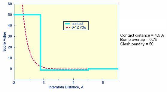
Distance
dependence of contact score function
The attractive score in grid is
negative and a
repulsive score is positive. This switch of sign is necessary to allow
the same minimization protocol to be used for contact scoring as
implemented for energy scoring.
Contact Grid Parameters
| Parameter |
Description |
Default Value |
| contact_score |
Flag to construct contact grid |
no |
| contact_cutoff_distance |
Maximum distance between heavy atoms for the interaction to be counted as a contact. |
4.5 |
RETURN TO TABLE OF CONTENTS
3.1.4. Energy
scoring
The energy scoring component of DOCK
is based on
the implementation of force field scoring. Force field scores are
approximate molecular mechanics interaction energies, consisting of van
der Waals and electrostatic components:
where each term
is a double sum over ligand atoms i and receptor atoms j, which include
the quantities listed below.
Generalization
of the VDW component
The van der Waals component of the
scoring
function has been generalized to handle any combination of repulsive
and attractive exponents (providing that a> b). The user may
choose
to "soften" the potential by using a 6-9 Lennard -Jones function. The
general form of the van der Waals interaction between two identical
atoms is presented:
where e is the well depth of the
interaction
energy, R is the van der Waals radius of the atoms, and coefficients C
and D can be determined given the two following boundary conditions:
 at
at

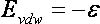 at
at
Application of these boundary
conditions to the
above equation yields an expression of the van der Waals interaction
with a generalized Lennard -Jones potential.
The consequence of using a different exponent for
the repulsive term is illustrated in Figure 1. Notice that the well
position and depth are unchanged, but that the repulsive barrier has
shrunk by about 0.25 angstrom.
Distance
dependence of the Lennard -Jones Function
Precomputing
potentials on a grid
By inspection of the above equations, the
repulsion and attraction parameters ( Aij and Bij ) for the
interactions of identical atoms can be derived from the van der Waals
radius, R, and the well depth, e.
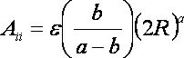
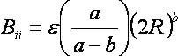
In order to evaluate the interaction energy
quickly, the van der Waals and electrostatic potentials are precomputed
for the receptor and stored on a grid of points containing the docking
site. Precomputing the van der Waals potential requires the use of a
geometric mean approximation for the A and B terms, as shown:
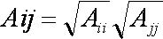
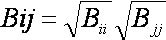
Using this approximation, the first
equation can be rewritten:
Three values are stored for every
grid point k
,each a sum over receptor atoms that are within a user defined cutoff
distance of the point:
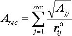
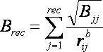
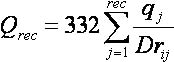
These values, with trilinear interpolation, are
multiplied by the appropriate ligand values to give the interaction
energy. Grid calculates the grid values and stores them in files. The
values are read in during a DOCK run and used for force field scoring.
The user determines the location and
dimensions of the grid box using the program showbox.
It is not necessary for the whole receptor to be enclosed; only the
regions where ligand atoms may be placed need to be included. The box
merely delimits the space where grid points are located, and does not
cause receptor atoms to be excluded from the calculation. Besides a
direct specification of coordinates, there is an option to center the
grid at a sphere cluster center of mass. Any combination of spacing and
x, y, and z extents may be used.
Energy Grid Parameters
| Parameter |
Description |
Default Value |
| energy_score |
Flag to perform energy scoring |
no |
| energy_cutoff_distance |
Maximum distance between two atoms for their contribution to the energy score to be computed. |
10 |
| atom_model |
Flag for how to model nonpolar hydrogens (u = United atom model, a = All atom model). |
u |
| attractive_exponent |
Exponent of attractive Lennard-Jones terms for VDW potential |
6 |
| repulsive_exponent |
Exponent of repulsive Lennard-Jones terms for VDW potential |
12 |
| distance_dielectric |
Flag to make the dielectric depend linearly on the distance. |
yes |
| dielectric_factor |
Coefficient of the dielectric |
4.0 |
RETURN TO TABLE OF CONTENTS
3.2. Docktools
Docktools is a
suite of programs that are available to create grids used by Dock3.5
score function in DOCK 6 which is an implementation of the
scoring function available in the older version of DOCK,
i.e., dock3.5.54. These programs can be used to generate steric,
electrostatic and
ligand and receptor desolvation grids. Dock3.5 scoring functionality
in DOCK 6 is an alternate scoring approach to electrostatic interaction
energy and also includes different grid-based methods for calculating
ligand and receptor desolvation. Docktools consists of chemgrid, solvmap, solvgrid (and sevsolv), grid-convert and
grid-convrds. This section will briefly review the
theory behind each of the programs
and describe the usage. The sevsolv program is included so that the chemgrid (dock3.5) scoring function matches DOCK 3.7 (or 3.8).
3.2.1.
CHEMGRID
AUTHOR: Brian K.
Shoichet
DESCRIPTION:
This program
chemgrid produces
values for computing force field scores and bump checking.
The force field
scores, or molecular mechanics interaction energies are calculated
as van der Waals and electrostatic components and stored on
grids.
The calculations are based on the theory presented in the Grid section
above. However only the steric interaction energy grids are used in
DOCK 6 as a part of Dock3.5 Score. The electrostatic interaction
calculation differs from Energy Scoring in the following aspects. For
calculating the electrostatic interaction, the electrostatic
potential of the receptor calculated using the linearized form of
Poisson-Boltzmann equation:

Where phi(x) the
potential is determined by the dielectric function epsilon(x), a
modified
Debye-Huckel parameter kappa(x), and the charge density of the receptor
rho(x). The electrostatic potential map (or phimap) is calculated using
DelPhi
and then is used by DOCK 6 to calculate the electrostatic interaction
energy as:
Where, qi
the partial charge of every atom i, is multiplied by the electrostatic
potential of the receptor phi at the respective atomic
position. Trilinear interpolation method is used for
interpolating the electrostatic potential from the phimap on to the
ligand position.
USAGE: chemgrid
INPUT FILE:
This programs require that an INCHEM
file be created in the working
directory, which contains the parameters to control the program. The
INCHEM parameters for chemgrid are detailed below:
receptor.pdb ; receptor pdb file
parameters/ prot.table.ambcrg.ambH ; charge parameter file
(for alternate naming conventions
see also prot.table.ambcrg.pdb3H, prot.table.ambcrg.pdbH,
and prot.table.ambcrg.sybH)
parameters/ vdw.parms.amb.mindock ; VDW parameter file
box.pdb ; box pdb file
0.33 ; grid spacing in angstroms
1 ; es type: distance-dependent dielectric; 2: constant dielectric
1 ; es scale for ff scoring
2.3 2.8 ; bumping distances for polar and non-polar receptor atoms
output_prefix ; output grid prefix name
OUTPUT FILES
- OUTCHEM #restatement of input
parameters; messages pertaining to calculation of the grids
- OUTPARM #messages pertaining to
parameterization of receptor atoms; net
charge on the receptor molecule including any ions or waters in the
receptor pdb file
- PDBPARM #shows which parameters
have been associated with each atom in the receptor pdb file
- output_prefix.bmp #bump grid
- output_prefix.vdw #vdw values for
receptor
- output_prefix.es #electrostatic
values for receptor
3.2.2
SOLVMAP
AUTHOR: Brian K. Shoichet
DESCRIPTION:
The solvmap program calculates the
grid that is used by DOCK6 for calculating ligand desolvation. Ligand
desolvation is calculated as a sum of the atomic desolvation multiplied
by a normalization factor that accounts for the extent to which the
ligand atom is buried by the binding site. The atomic desolvation for
each ligand atom can be calculated by AMSOL (AMSOL is not distributed by us, please follow the link for more information) and is stored in the
input file (see file formats). The cost of desolvating each atom, or
the normalization factor, is the distance weighted high dielectric
volume displaced by the protein that
is stored for each grid element in the active site. Thus the volume based ligand desolvation energy is calculated as:
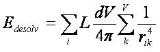
Here L is the ligand atom desolvation, volume summed over k volume elements, V.
This method is only an approximation to GB solvation and works within
the limits of complete burial from the solvent and complete exposure to
the solvent on the protein surface. However, being grid-based it is
fast and can be used during conformational search and final scoring.
USAGE: solvmap
INPUT FILE:
This programs require that an INSOLV
file be created in the working
directory, which contains the parameters to control the program. The
INSOLV parameters for chemgrid are detailed below:
receptor.pdb; receptor file
solvmap ;
output grid file
1.4,1.3,1.7,2.2,2.2,1.8 ; radii of oxygen, nitrogen, carbon,
sulfur, phosphorus, and "other" atoms.
1.4
; radius of probe
1
; grid resolution
box.pdb
; box file
OUTPUT FILES:
- OUTSOLV
#restatement of input parameters; messages pertaining to calculation of
the grids
- solvmap #ligand desolvation grids
Starting in 6.11, The solvmap program program from DOCK 3.7 is also now included and is called solvmapsev (MySinger, J Chem Inf Model 2010).
3.2.3
SOLVGRID
AUTHOR Kaushik Raha
DESCRIPTION:
The solvgrid program creates bulk
(or receptor) and explicit (or ligand) desolvation grids using the
occupancy desolvation method (Luty et. al., J. Comp. Chem, 1995; Verkhiver et. al., J. Mol. Recog., 1999). The occupancy desolvation
method is phenomenological in nature where desolvation energy can be
described pairwise additively. The desolvation energy due to
interaction between a ligand atom and receptor atom can be calculated
as the solvent affinity of a ligand atom weighted by the
volume of the solvent displaced from the receptor atom due to binding
and vice versa. Thus,
Edsol = Si ϕDES,EXPL(xi)
+ fi
ϕDES,BULK(xi)
Where the mobile atom i, has a solvation affinity of Si
and a fragmental volume of fi.
The solvent affinity of the ligand atom is calculated as:

Where qi
is the charge on the ligand atom i,
and alpha and beta are constants set at alpha = 0.25 kcal/mol
and beta = -0.005 kcal/mol.
fi is the volume of ligand atom i,
calculated from the amber radius of the ligand atom. For the receptor,
these can be precalculated and stored on a grid. ϕDES,BULK(xi)
and ϕDES,EXPL(xi)
are interpolated from grids calculated using the solvgrid program
during docking. It requires the calculation of two separate
grids:
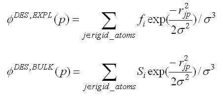
where j is a rigid receptor
atom, and Sj
and fj
are the solvent affinity and the fragmental volume of the receptor atom
respectively. Bulk and explicit desolvation grids are calculated from fj
and Sj
at grid points p,
distance rjp
from the receptor atom multiplied by Gaussian weighting of the
distance. The solvgrid program calculates these grids from
the charge and the volume of the receptor atoms.
USAGE: solvgrid
INPUT
This programs require that an INRDSL
file be created in the working
directory, which contains the parameters to control the program. The
INRDSL parameters for solvgrid are detailed below:
receptor.pdb ; receptor pdb file
parameters/ prot.table.ambcrg.ambH ; charge parameter file<
(for alternate naming conventions
see also prot.table.ambcrg.pdb3H, prot.table.ambcrg.pdbH,
and prot.table.ambcrg.sybH)
parameters/ vdw.parms.amb.mindock ; VDW parameter file
box.pdb ; box pdb file
0.33 ; grid spacing in angstroms
1 ; es type: distance-dependent dielectric; 2: constant dielectric
4 ; es scale for ff scoring
2.3 2.8 ; bumping distances for polar and non-polar receptor atoms
output_prefix ; output grid prefix name
sol_op ; method for calculating desolvation grid
solE_recep; solvation free energy of receptor
OUTPUT FILES
- OUTRDSL #restatement of input
parameters; messages pertaining to calculation of the grids
- OUTPARM #messages pertaining to
parameterization of receptor atoms; net
charge on the receptor molecule including any ions or waters in the
receptor pdb file
- PDBPARM #shows which parameters
have been associated with each atom in the receptor pdb file
- output_prefix.bmp #bump grid
- output_prefix.vdw #vdw values for
receptor
- output_prefix.es #electrostatic
values for receptor
- output_prefix.dsl #bulk and
explicit desolvation grid for receptor
3.2.4
GRID-CONVERT
AUTHOR: Kaushik Raha, John J. Irwin
(Derived from Todd Ewing's GRID Program)
DESCRIPTION:
This consists of programs
grid-convert and grid-convrds that convert grids generated by chemgrid,
solvgrid and DelPhi into DOCK6 readable grids.
Note that grids created by program Grid
are already DOCK6 readable grids. Thus, even though the input of
grid-convert may contain parameters related to Grid
produced grids, such grids do not need conversion - to wit the contact grid.
Update grid-convert. Updated grid-convert to convert qnifft grids and to convert grid generated with blastermaster.py from DOCK3.7. (Balius, J.Comput. Chem. 2024)
USAGE: grid-convert -i gconv.in
>& gconv.out
INPUT FILES:
gconv.in;
input file with parameters
vdw.defn;
vdw parameters file
conv.defn;
atomtype definition file
RETURN TO TABLE OF
CONTENTS
3.3. Nchemgrids
AUTHOR: Xiaoqin
Zou
USAGE:
nchemgrid_GB or nchemgrid_SA
INPUT FILE:
Both programs require that an INCHEM
file be
created in the working directory, which contains the parameters to
control the program. The INCHEM parameters for both the nchemgrid_GB
and nchemgrid_SA programs are detailed below:
For
nchemgrid_GB:
receptor.pdb ; receptor pdb file
cavity.pdb ; cavity pdb file
parameters/ prot.table.ambcrg.ambH ; charge parameter file
(for alternate naming conventions
see also prot.table.ambcrg.pdb3H, prot.table.ambcrg.pdbH,
and prot.table.ambcrg.sybH)
parameters/ vdw.parms.amb ; VDW parameter file
box.pdb ; box pdb file
0.4 ; grid spacing in angstroms
2 ; es type: GB
1 ; es scale for ff scoring
8.0 8.0 ; cutoff for es and outer box
78.3 78.3 ; dielectric of solvent ,cavity
2.3 2.8 ; bumping distances
output_prefix ; output grid prefix name
1 ; pairwise calculation
NOTE: The cavity.pdb file should be
an empty
file. This feature is not frequently used. However, the parameter must
still be passed. The pairwise calculation value must also always be 1.
For nchemgrid_SA:
receptor.pdb ; receptor pdb file
parameters/prot.table.ambcrg.ambH ; charge parameter file
(for alternate naming conventions
see also prot.table.ambcrg.pdb3H, prot.table.ambcrg.pdbH,
and prot.table.ambcrg.sybH)
parameters/ vdw.parms.amb ; VDW parameter file
box.pdb ; box pdb file
0.4 ; grid spacing in angstroms
1.4 ; probe radius for SA
2 ; scoring type: SA
8.0 ; cutoff for SA calculations
output_prefix ; output grid prefix name
DESCRIPTION:
The nchemgrid_gb and nchemgrid_sa
programs create the GB and SA receptor grids for use with the Zou GB/SA
scoring function (see Zou GB/SA Scoring).
OUTPUT FILES
For nchemgrid_gb
- inva #debugging
file with inverse Born radius for receptor atoms
- NEG_INVA #error file listing
embedded receptor atoms
- OUTCHEM #restatement of input
parameters; messages pertaining to calculation of the grids
- OUTPARM #messages pertaining to
parameterization of receptor atoms; net charge on the receptor molecule
including any ions or waters in the receptor pdb file
- PDBPARM #shows which parameters
have been associated with each atom in the receptor pdb file
screen.para #file that contains descreening parameters
- zou_grid.bmp #bump grid
- zou_grid.rec #xyz coordinates,
effective
charge, effective vdw radii, inverse Born radii, and descreening
parameters for receptor
- zou_grid.sol #flags for whether
receptor atoms are solvated
- zou_grid.vdw #vdw values for
receptor
For
nchemgrid_sa:
- OUTCHEM
#restatement of input parameters; messages pertaining to calculation of
the grids
- OUTPARM #messages pertaining to
parameterization of receptor atoms; net charge on the receptor molecule
including any ions or waters in the receptor pdb file
- PDBPARM #shows which parameters
have been associated with each atom in the receptor pdb file
- zou_grid.bmp #bump grid
- zou_grid.sas #xyz coordinates,
effective vdw
radii, vdw type, number of spherical grid points, and polarity type for
each receptor atom
- zou_grid.sasmark
#information about grid spacing, coordinates, dimensions, etc
RETURN TO TABLE OF CONTENTS
3.4. Sphgen
AUTHOR: Irwin D.
Kuntz (modified by Renee DesJarlais and Brian Shoichet)
USAGE: sphgen
INPUT FILE*:
rec.ms #molecular surface file
R #sphere outside of surface (R) or inside surface (L)
X #specifies subset of surface points to be used (X=all points)
0.0 #prevents generation of large spheres with close surface contacts
(default=0.0)
4.0 #maximum sphere radius in angstroms (default=4.0)
1.4 #minimum sphere radius in angstroms (default=radius of probe)
rec.sph #clustered spheres file
*WARNINGS:
(1) The input file names and parameters are read from a file called
INSPH, which should not contain any blank lines or the comments
(denoted by # ) from above.
(2) The molecular surface file must include surface normals. Sphgen
expects the Fortran format
A3, I5, X, A4,
X, 2F8.3, F9.3, X, A3, 7X, 3F7.3
DESCRIPTION:
3.4.1. Overview
Sphgen generates sets of overlapping spheres to
describe the shape of a molecule or molecular surface. For receptors, a
negative image of the surface invaginations is created; for a ligand ,
the program creates a positive image of the entire molecule. Spheres
are constructed using the molecular surface described by Richards
(1977) calculated with the program
dms .
Each sphere touches the molecular surface at two points and has its
radius along the surface normal of one of the points. For the receptor,
each sphere center is outside the surface, and lies in the direction of
a surface normal vector. For a ligand, each sphere center is inside the
surface, and lies in the direction of a reversed surface normal vector.
Spheres are calculated over the entire surface,
producing approximately one sphere per surface point. This very dense
representation is then filtered to keep only the largest sphere
associated with each receptor surface atom. The filtered set is then
clustered on the basis of radial overlap between the spheres using a
single linkage algorithm. This creates a negative image of the receptor
surface, where each invagination is characterized by a set of
overlapping spheres. These sets, or clusters, are sorted according to
numbers of constituent spheres, and written out in order of descending
size. The largest cluster is typically the ligand binding site of the
receptor molecule. The program showsphere writes out sphere center
coordinates in PDB format and may be helpful for visualizing the
clusters (see showsphere).
RETURN TO TABLE OF CONTENTS
3.4.2.
Critical Points
The process of labeling site
points for critical matching must currently be done by hand (see Critical Points
for use in DOCK). The user should load the site points and the receptor
coordinates into a graphic program to determine the spheres closest to
the target area. Once a sphere or group of spheres has been determined
to be critical, the sphere(s) should be labeled by changing the second
to last column of the final sphere file to the critical cluster number
(see Output).
RETURN TO TABLE OF CONTENTS
3.3.3.
Chemical Matching
The process of labeling site
points for chemical matching must also be done by hand (see Chemical Matching
for use in DOCK). The user should load the site points and the receptor
coordinates into a graphic program and study the local environment of
each point. Labeled site points may be input as either a SPH format or
SYBYL MOL2 format coordinate file. To store labeled site points in a
MOL2 file, select an atom type for each label of interest. Then edit
the chem.defn file to include the selected atom types (see chem.defn).
Site point definitions can be distinguished from ligand atom
definitions by explicitly requiring that no bonded atoms can be
attached (ie. followed by [*]). Using the convention in that example
file, site points should be labeled as follows: hydrophobic, "C.3";
donor, "N.4"; acceptor, "O.2"; polar, "F".
Example
of chemical labels in SPH format
DOCK 3.5 receptor_spheres
color hydrophobic 1
color acceptor 2
color donor 3
cluster 1 number of spheres in cluster 49
7 2.34500 36.49000 16.93500 1.500 0 0 1
8 -0.05200 42.29900 14.18800 1.500 0 0 1
9 -0.67000 41.20600 11.59800 1.500 0 0 1
17 -6.00000 34.00000 17.00000 1.500 0 0 3
18 -5.00000 29.00000 22.00000 1.500 0 1 3
...
Caveats
on Chemical Matching
It can take a significant amount
of effort to
chemically label a large site and to verify that the docking results
are what were expected. If you use this chemical matching, plan to
spend some time in preparation and validation BEFORE running an entire
database of molecules.
It must be pointed out that the ultimate
arbiter of which orientations of a ligand are saved is actually the
scoring function. If the scoring function is unable to discriminate
what the user feels are bad chemical interactions, then any improvement
with chemical matching will probably be obscured. In addition, if score
optimization is used, then the orientation will be perturbed from the
original chemically-matched position to a new score-preferred
positions.
RETURN TO TABLE OF CONTENTS
3.4.4. Output
Some informative messages are
written to a file
called OUTSPH. This includes the parameters and files used in the
calculation. The spheres themselves are written to the clustered
spheres file. They are arranged in clusters with the cluster having the
largest number of spheres appearing first. The sphere cluster file
consists of a header followed by a series of sphere clusters. The
header is the line DOCK 3.5 receptor_spheres followed by a color table
(see Chemical Matching).
The
color table contains color names each on a separate line. As sphgen
produces no colors, the color table is simply absent.
The sphere clusters themselves
follow, each of which starts with the line
cluster n
number of spheres in cluster i
where n is the cluster number for
that sphere
cluster, and i is the number of spheres in that cluster. Next, all
spheres in that cluster are listed in the format below:
FORMAT: (I5, 3F10.5, F8.3, I5,
I2, I3)
I: Integer F: Float
012345012345678901234567890123456789012345678901234567890123456789
63 5.58405 50.91005 59.97029 1.411 92 0 0
64 9.00378 52.46159 62.30926 1.400 321 0 0
66 11.43685 56.49715 61.79008 1.984 493 0 0
I5: Column 0~4 (the first 5 columns) were used to put integer data.
F10.5: Column 5~14 (total 10 columns, and 5 digits for mantissa) were
used to put float data.
The values in the sphere file
correspond to:
- The number of the atom with
which surface point i (used to generate the sphere) is associated.
- The x, y ,and z coordinates of
the sphere center.
- The sphere radius.
- The number of the atom with
which surface point j (second point used to generate the sphere) is
associated.
- The critical cluster to which
this sphere belongs.
- The sphere color. The color is simply an
index into the color table that was specified in the header. Therefore,
1 corresponds to the first color in the header, 2 for the second, etc.
0 corresponds to unlabeled.
The clusters are listed in numerical
order from
largest cluster found to the smallest. At the end of the clusters is
cluster number 0. This is not an actual sphere cluster, but a list of
all of the spheres generated whose radii were larger than the minimum
radius, before the filtering heuristics ( i.e., allowing only one
sphere per atom and using a maximum radius cutoff) and clustering were
performed. Cluster 0 may be useful as a starting point for users who
want to explore a wider range of possible clusters than is provided by
the standard sphgen clustering routine. The program creates three
temporary files: temp1.ms, temp2.sph, and temp3.atc. These are used
internally by sphgen, and are deleted upon completion of the
computation. For more information on sphere generation and selection,
go to the
Sphere Generation and Selection demo.
RETURN TO TABLE OF CONTENTS
3.5. Showbox
AUTHOR: Elaine Meng
USAGE: showbox [< input.in]
DESCRIPTION:
Showbox is an interactive program for specifying
the location and the size of the grids that will be
calculated by the program grid. The output is in PDB format and
thus can be visualized with many graphics programs.
The user is asked whether the box should be
automatically constructed to enclose all of the spheres in a cluster.
If so, the user must also enter a value for how closely the box faces
may approach a sphere center (how large a cushion of space is desired)
and the sphere cluster filename and number. If not, the user is asked
whether the box will be centered on manually entered coordinates or a
sphere cluster center of mass. Depending on the response, the
coordinates of the center or the sphere cluster filename and number are
requested. Finally, the user must enter the desired box dimensions (if
not automatic) and a name for the output PDB-format box file. If the
input parameters are known, they can be listed in an input file and
redirected into the program.
For a flowchart of the input tree and an example input, see STEP 1 of the
Grid Generation Tutorial.
See also the discussion of
showbox in the grid energy scoring section.
RETURN TO TABLE OF CONTENTS
3.6. Showsphere
AUTHORS: Stuart
Oatley , Elaine Meng , Daniel Gschwend
USAGE:
showsphere [< input.in]
DESCRIPTION:
Showsphere is an interactive program; it produces
a PDB-format file of sphere centers and an MS-like file of sphere
surfaces, given the sphere cluster file and cluster number. The surface
file generation is optional. The user may specify one cluster or all,
and multiple output files will be generated, with the cluster number
appended to the end of the name of each file. The input cluster file is
created using sphgen (see sphgen).
Showsphere
requests the name of the sphere cluster file, the number of the cluster
of interest, and names for the output files. Information is sent to the
screen while the spheres are being read in, and while the surface
points are being calculated. If the input parameters are known, they
can be listed in an input file and piped into the program.
RETURN TO TABLE OF CONTENTS
3.7. Sphere Selector
AUTHOR: P. Therese Lang
USAGE:
sphere_selector < sphere_cluster_file.sph >
<set_of_atoms.mol2> <radius>
DESCRIPTION:
Sphere_selector filters the output from
sphgen selecting all spheres within a
user-defined radius of a target molecule (see sphgen).
The target molecule can be anything (e.g., known ligand or receptor residue)
as long as it is in proper MOL2 format. WARNING: Please note that
above order of input files must be maintained for the program to work.
The total number of spheres is unlimited, eliminating the
maximum of 100000 spheres in versions prior to DOCK 6.1.
RETURN TO TABLE OF CONTENTS
3.8. Antechamber
Antechamber
is an accessory program originally developed to prepare small molecules
on the fly to use in AMBER. With permission, we have included a
distribution of the code to facilitate preparing small molecules for
Amber score.
For more information on the use of the antechamber accessory,
please visit the source web site at
ambermd.org/antechamber/antechamber.html.
From the web site:
"Antechamber
is a set of auxiliary programs for molecular mechanic (MM) studies.
This software package is devoted to solve the following problems during
the MM calculations: (1) recognizing the atom type; (2) recognizing
bond type; (2) judging the atomic equivalence; (3) generating residue
topology file; (4) finding missing force field parameters and supplying
reasonable and similar substitutes. As an accessory module...,
antechamber can generate input automatically for most organic molecules
in a database...."
RETURN TO TABLE OF CONTENTS
3.9. tLEaP
tLEaP is an accessory program
that provides for basic model building and Amber coordinate and
parameter/topology input file creation.
For more information see the AmberTools distribution:
ambermd.org/.
tleap is only used during the preparation for Amber Score.
tleap's charge tolerance has been increased from 0.0001 (as in Amber10) to
0.001 to avoid excessive instances of left over charges of plus or minus one.
RETURN TO TABLE OF CONTENTS
3.10.
Amber Score Preparation Scripts
AMBER score requires many additional input files beyond those of
other DOCK scoring functions; see
AMBER Score Inputs
for more information.
All the input files, such as the prmtop, frcmod, amber.pdb, etc.
should be generated prior to running the DOCK AMBER score.
Two perl scripts, prepare_amber.pl and prepare_rna_amber.pl, have
been provided for this purpose.
The script prepare_rna_amber.pl differs from prepare_amber.pl
in that the former treats all nucleic acids as RNA
whereas the latter treats them as DNA; in addition,
prepare_rna_amber.pl supports the RNA specific features
to neutralize to a total charge of zero
and to solvate with water.
The script prepare_amber.pl performs the following
main tasks:
(i) Reads the PDB file for the receptor;
adds hydrogens and some other missing atoms if not present;
adds AMBER force field atom types and charges. Generates Amber
parameter/topology (prmtop) and coordinate (inpcrd) files.
This is performed via the script amberize_receptor which invokes
program tleap.
(ii) Generates a modified mol2 file with suffix amber_score.mol2
(e.g., lig.amber_score.mol2) that appends to each TRIPOS MOLECULE a
TRIPOS AMBER_SCORE_ID section containing a unique label
(e.g., lig.1, mydnagil.1, etc.).
This modified mol2 file should be assigned to the ligand_atom_file
input parameter in the DOCK input file.
(iii) Splits the ligand_mol2_file into separate mol2 files,
one file per ligand, where the file prefixes are the AMBER_SCORE_ID
unique labels. These mol2 files are used in the next step.
(iv) Runs the antechamber program to determine the semi-empirical charges,
such as AM1-BCC, for each ligand. Runs the tleap program to create
parameter/topology and coordinate files for each ligand using the
GAFF force field (prmtop, frcmod, and inpcrd),
and writes a mol2 file for the ligands with GAFF atom types (gaff.mol2).
This is performed via the script amberize_ligand.
(v) Combines each ligand with the receptor to generate the parameter/topology
and coordinate files for each complex.
This is performed via the script amberize_complex which invokes
program tleap.
The script prepare_amber.pl also creates files
with extensions .log and .out that contain the detailed results of the above
steps. The amberize_*.out files can be browsed to verify that the
preparation was successful. If prepare_amber.pl emits any warnings
or errors then all these files should be scrutinized.
Some errors are fatal, such as an inability to prepare the receptor;
generally, and in this case especially
start investigating by examining file amberize_receptor.out.
Since preparation for Amber score is more stringent than
preparation for other DOCK scores, usually a small fraction
of a large set of ligands fails during prepare_amber.pl execution. This
DOCK-Fans post
discusses in detail the recovery options for failing ligands.
See the
tutorials
for a complete example usage. Two options not discussed in the tutorial
are designed for rescoring large ligand databases and should be applied
only after experience with small data sets. These options are to use
the existing ligand charges and to ignore non-receptor related errors.
In addition, for DOCKing ligands to RNA the script prepare_rna_amber.pl
supports neutralizing to a total charge of zero and solvating with water.
Here are the man pages for prepare_amber.pl and prepare_rna_amber.pl.
- prepare_amber.pl
AUTHORS: Devleena Shivakumar and Scott Brozell
USAGE:
prepare_amber.pl [-c] [-i] DOCK_ranked_mol2_file Receptor_PDB_file
OPTIONS:
-c
Use charges from the DOCK_ranked_mol2_file.
The default behavior is to generate AM1-BCC charges.
This option must occur before DOCK_ranked_mol2_file.
-i
Ignore errors during ligand and complex amberization.
Errors during receptor amberization still cause abortion.
The default behavior is to abort on all errors.
This option must occur before DOCK_ranked_mol2_file.
DESCRIPTION:
Create Amber input files from a mol2 file containing DOCKed ligands
and from a pdb file containing the receptor consisting of protein or DNA.
In particular, any nucleic acids are assumed to be DNAs.
The Amber input files are necessary for the DOCK Amber Score.
- prepare_rna_amber.pl
AUTHORS: Devleena Shivakumar and Scott Brozell
USAGE:
prepare_rna_amber.pl [-c] [-i] [-n] [-s] DOCK_ranked_mol2_file Receptor_PDB_file
OPTIONS:
-c
Use charges from the DOCK_ranked_mol2_file.
The default behavior is to generate AM1-BCC charges.
This option must occur before DOCK_ranked_mol2_file.
-i
Ignore errors during ligand and complex amberization.
Errors during receptor amberization still cause abortion.
The default behavior is to abort on all errors.
This option must occur before DOCK_ranked_mol2_file.
-n
Neutralize to a total charge of zero by adding sodium and
chloride ions. The default is no neutralization.
This option must occur before DOCK_ranked_mol2_file.
-s
Solvate with water via LEaP's solvateoct x TIP3PBOX 5.0.
The default is no solvation.
This option must occur before DOCK_ranked_mol2_file.
DESCRIPTION:
Create Amber input files from a mol2 file containing DOCKed ligands
and from a pdb file containing the receptor consisting of protein or RNA.
In particular, any nucleic acids are assumed to be RNAs.
The Amber input files are necessary for the DOCK Amber Score.
Under the best conditions these prepare scripts will work
as designed, but if not then here is a starting point for
looking under the hood.
- amberize_receptor
AUTHORS: Scott Brozell and Dave Case
USAGE:
amberize_receptor [-k] [-n] [-r] [-s] receptor_pdb_file_prefix
Execute the command without input for more details.
DESCRIPTION:
Create Amber input files from a pdb file containing only the receptor.
The Amber input files are necessary for the DOCK Amber Score.
- amberize_ligand
AUTHORS: Scott Brozell, Dave Case, and
Devleena Shivakumar
USAGE:
amberize_ligand [-k] ligand_mol2_file_prefix [antechamber_charge_options]
Execute the command without input for more details.
DESCRIPTION:
Create Amber input files from a mol2 file containing only the ligand
and from an optional specification of the Antechamber charge treatment.
The Amber input files are necessary for the DOCK Amber Score.
- amberize_complex
AUTHORS: Scott Brozell and Dave Case
USAGE:
amberize_complex [-k] [-n] [-r] [-s] receptor_name ligand_name
Execute the command without input for more details.
DESCRIPTION:
Create Amber input files from an Amber compatible pdb file containing
only the receptor, which is usually produced from amberize_receptor,
and from an Amber compatible mol2 file containing only the ligand,
which is usually produced from amberize_ligand.
The Amber input files are necessary for the DOCK Amber Score.
RETURN TO TABLE OF CONTENTS
Molecular
File Formats
RETURN TO TABLE OF CONTENTS
4.1. Tripos MOL2 Format
This format is used for general
molecule input and output of DOCK. Although previous versions of DOCK
supported an extended PDB format to store molecule information, the
current version now uses MOL2 as the molecule format. This format has
the advantage of storing all the necessary information for atom
features, position, and connectivity. It is also a standardized format
that other modeling programs can read. For more information on how to
generate MOL2 files from PDB files, go to the
Structure Preparation demo.
Of the many record types in a MOL2 file, DOCK recognizes the following:
MOLECULE, ATOM, BOND, SUBSTRUCTURE and SET. In the MOLECULE record,
DOCK utilizes information about the molecule name and number of atoms,
bonds, substructures and sets. In the ATOM record DOCK utilizes
information about the atom names, types, coordinates, residue numbers, and
partial charges. In the BOND record, DOCK utilizes the atom identifiers for the
bond. In the SUBSTRUCTURE record, DOCK records the fields, but does not
utilize them. The SET records are entirely optional. They are used only
in special circumstances, such as for ligand flexibility.
In DOCK 6, additional record types have been introduced. One is the
SOLVATION record that has the atomic desolvation information for the
ligand atoms. The parameter read_mol_solvation can be used to read in
this record.
Another is the AMBER_SCORE_ID record that is used by AMBER score.
This record should be appended to each TRIPOS MOLECULE and should
contain a unique label for that ligand. This type of modified mol2 file
is required by AMBER score and its name should be assigned to the
ligand_atom_file input parameter in the DOCK input file.
To facilitate analysis of docking results, the header section of mol2 files
written out by DOCK will contain fields, preceded by multiple #### signs,
with relevant docking components (i.e. descriptors). For example, docking
energies, their components, rmsd values, pharmacophore overlap, and footprint
similarity, among others, will be written to file depending on which scoring
function(s) were used.
The Chimera program
ViewDock
tool can be used to load a DOCK multi-mol2 files containing various descriptors
which can be examined in the ViewDock ListBox. This can be a useful way
to prioritize subsets of compounds from a large virtual screen. ListBox descriptors
can easily be sorted which facilities the isolation of compounds with
user-favored properties.
For extensive
details on the MOL2 format, as well as example files, please refer to
the archived Tripos documentation
(Tripos-mol2.pdf).
RETURN TO TABLE OF CONTENTS
4.2. PDB Format
This format is used for several of
the DOCK accessories and the AMBER score function. For extensive
details on the PDB format, as well as example files, please refer to
the Protein Databank File Format Documentation (http://www.pdb.org/pdb/static.do?p=file_formats/pdb/index.html).
RETURN TO TABLE OF CONTENTS
4.3. BILD Format
This format is used to visualize the directional vectors in pharmacophore models generated by the FMS protocol using the molecular modeling software Chimera. Please refer to the UCSF Computer Graphics Laboratory BILD format documentation(http://www.cgl.ucsf.edu/chimera/docs/UsersGuide/bild.html).
First, the following DOCK input parameters need to be set. By default, the parameters "*_write_out_reference_ph4", "*_write_out_candidate_ph4" and "*_write_out_matched_ph4" or are set to "no" and no output pharmacophore mol2 file will be generated.
For FMS alone scoring protocol:
- fms_score_write_reference_pharmacophore_txt yes
- fms_score_reference_output_mol2_filename ref_ph4.mol2
- fms_score_write_candidate_pharmacophore yes
- fms_score_candidate_output_filename cad_ph4.mol2
- fms_score_write_matched_pharmacophore yes
- fms_score_matched_output_filename mat_ph4.mol2
For using FMS score in the descriptor scoring function:
- descriptor_fms_score_write_reference_pharmacophore_txt yes
- descriptor_fms_score_reference_output_mol2_filename ref_ph4.mol2
- descriptor_fms_score_write_candidate_pharmacophore yes
- descriptor_fms_score_candidate_output_filename cad_ph4.mol2
- descriptor_fms_score_write_matched_pharmacophore yes
- descriptor_fms_score_matched_output_filename mat_ph4.mol2
In the pharmacophore output mol2 files "ref_ph4.mol2", "cad_ph4.mol2" and "mat_ph4.mol2", each pharmacophore point is represented by a set of atoms (Table X, column c). Note for HBD, HBA, ARO and RNG labeled pharmacophore points, more than one atom is used because both the center of the point (denoted by the first atom in the list) and the directionality (derived from all the atoms in the list) need to be recorded. The output pharmacophore mol2 file will then be converted to a bild file using a python script mol2bild.py (can be found in the DOCK bin directory). The bild file contains the directional vectors derived for all the pharmacophore points with directionality (HBD, HBA, ARO, RNG) in the original mol2 file. Different colors are used to represent different pharmacophore labels as shown in Table X column d. The directional vectors are modeled as 3D arrow geometric objects in the molecular modeling software Chimera, each consists of a cylinder (from the start point to an intermediary point) and a cone (from the intermediary point to the end point) representing the arrowhead. As an example, a 3D arrow for a ring pharmacophore feature is written as follows in the bild file.
.color orange
.arrow    0.64  -17.12  -10.61    0.99  -17.69   -9.86 0.01 0.04 0.75
.color orange
.arrow    0.64  -17.12  -10.61    0.30  -16.55  -11.36 0.01 0.04 0.75
.color orange
.arrow   -0.04  -15.65   -9.18    0.30  -16.22   -8.43 0.01 0.04 0.75
.color orange
.arrow   -0.04  -15.65   -9.18   -0.39  -15.09   -9.93 0.01 0.04 0.75
.color orange
.arrow   -0.22  -16.30   -4.16   -0.73  -16.46   -3.32 0.01 0.04 0.75
.color orange
.arrow   -0.22  -16.30   -4.16    0.29  -16.15   -5.01 0.01 0.04 0.75
.color orange
.arrow   -1.30  -14.47   -4.50   -1.81  -14.62   -3.65 0.01 0.04 0.75
.color orange
.arrow   -1.30  -14.47   -4.50   -0.79  -14.33   -5.35 0.01 0.04 0.75
.color red
.arrow   -7.12  -15.42   -2.60   -7.25  -14.95   -1.73 0.01 0.04 0.75
.color red
.arrow   -7.11  -15.54   -4.81   -7.24  -15.16   -5.73 0.01 0.04 0.75
.color blue
.arrow    2.65  -16.61  -11.14    1.71  -16.86  -10.90 0.01 0.04 0.75
.color blue
.arrow    1.53  -15.84  - 3.04    0.72  -16.07   -3.57 0.01 0.04 0.75
Here, each Chimera object is defined by two lines. The first line defines the color of the Chimera object (e.g. ".color orange"). The second line defines the type of the geometric object (".arrow"), the start and end point of the arrow ( (x1, y1, z1)= (0.64, -17.12, -10.61) and (x2, y2, z2)= (0.99, -17.69, -9.86) in the first object in the above example, arrow pointing from (x1, y1, z1) to (x2, y2, z2) ), as well as the size of the arrow (radius of the cylinder r1= 0.01, the radius of the base of the cone r2=0.04, and the ratio of the length of cylinder to that of the complete arrow rho=0.75).
Pharmacophore feature representation in ph4.mol2 and ph4.bild
|
a. Label
|
b. definition
|
c. mol2
|
d. bild
|
|
PHO
|
Hydrophobic
|
C
|
-
|
|
HBD
|
Hydrogen bond donor
|
HD, N
|
blue
|
|
HBA
|
Hydrogen bond acceptor
|
O, HA
|
red
|
|
ARO
|
Aromatic ring
|
S, H1, H2
|
orange
|
|
RNG
|
Non-aromatic ring
|
P, H3, H4
|
yellow
|
|
POS
|
Positively charged
|
Na
|
-
|
|
NEG
|
Negatively charged
|
Cl
|
-
|
The complete bild file includes all the directional vectors derived from the pharmacophore mol2 files. Both the pharmacophore mol2 and bild files will be opened in Chimera for visualization of the pharmacophore model.
RETURN TO TABLE OF CONTENTS
References
Allen, W.J., Rizzo, R.C.
Implementation of the Hungarian Algorithm to Account for Ligand Symmetry
and Similarity in Structure-Based Design. J. Chem. Inf. Model. 54:518-529, 2014.
Allen, W.J.; Balius, T.E.;
Mukherjee, S.; Brozell, S. R.; Moustakas, D. T.; Lang, P. T.; Case, D. A.;
Kuntz, I. D.; Rizzo, R. C. DOCK 6: Impact of New Features and Current
Docking Performance. J. Comput. Chem. 36(15): 1132-1156, 2015.
Allen, W.J.; Fochtman, B.C.;
Balius, T.E.; Rizzo, R.C. Customizable de novo design strategies for DOCK: Application to
HIVgp41 and other therapeutic targets J. Comput. Chem. 38(30): 2641-2663, 2017.
Balius, T.E., Mukherjee, S.,
and Rizzo, R.C., Implementation and Evaluation of a Docking-Rescoring Method
using Molecular Footprint Comparisons. J. Comput. Chem. 32(10): 2273-2289, 2011.
Balius, T.E., Allen, W.J.,
Mukherjee, S. and Rizzo, R.C. Grid-based Molecular Footprint Comparison
Method for Docking and De Novo Design: Application to HIVgp41. J. Comput.
Chem. 34(14): 1226-1240, 2013.
Balius, T.E.,
Tan, Y.S., Chakrabarti, M., DOCK 6: Incorporating hierarchical traversal
through precomputed ligand conformations to enable large-scale docking.
J. Comput. Chem. 45(1): 47-63, 2024.
https://doi.org/10.1002/jcc.27218
Balius, T. E., Fischer, M.,
Stein, R. M., Adler, T. B., Nguyen C. N., Cruz A., Gilsonc M. K., Kurtzman,
T., Shoichet, B. K., Testing inhomogeneous solvation theory in structure-based
ligand discovery. Proc. Natl. Acad. Sci. USA., 114 (33): E6839-E6846, 2017
Bender, A., Mussa, H.Y.,
Glen, R.C., Reiling, S. Similarity Searching of Chemical Databases Using
Atom Environment Descriptors (MOLPRINT 2D): Evaluation of Performance.
J. Chem. Inf. Comput. Sci. 2004, 44, 1708.
Bickel, J. D., Boysan, B. T.,
Rizzo, R. C. Fragment and torsion biasing algorithms for construction of small
organic molecules in proteins using DOCK. J. Comput. Chem. 2025 46, e27508.
Brozell, S.R., Mukherjee, S.,
Balius, T.E., Roe, D.R., Case, D.A., Rizzo, R.C., Evaluation of DOCK 6 as
a Pose Generation and Database Enrichment Tool. J. Comput. Aided Mol. Design.
26(6): 749-773, 2012.
Coleman, R.G., Carchia, M.,
Sterling, T., Irwin, J.J., Shoichet, B.K., Ligand Pose and Orientational
Sampling in Molecular Docking. PLOS ONE 8(10): e75992, 2013.
Deb, K.; Pratap, A.; Agarwal, S.;
Meyarivan, T. A fast and elitist multiobjective genetic algorithm: NSGA-II.
IEEE Transactions on Evolutionary Computation. 6: 182-97, 2002.
DesJarlais, R.L. and Dixon, J.S. A Shape-and chemistry-based docking method
and its use in the design of HIV-1 protease inhibitors. J. Comput-Aided Molec.
Design. 8: 231-242, 1994.
Ewing, T. J. A.; Makino, S.; Skillman, A. G.; Kuntz, I. D.
DOCK 4.0: search strategies for automated molecular docking of
flexible molecule databases.
J. Comput-Aided Molec. Design. 15: 411-428 (2001).
Ewing,
T.J.A. and Kuntz, I.D., Critical evaluation of search algorithms for
automated molecular docking and database screening. J. Comput. Chem.
18: 1175-1189, 1997.
Ferro,
D.R. and Hermans, J. Different best rigid-body molecular fit routine.
Acta. Cryst. A. 33: 345-347, 1977.
Graves, A.P., Shivakumar, D.M., Boyce, S.E., Jacobson, M.P., Case, D.A. and
Shoichet, B.K. Rescoring Docking Hit Lists for Model Cavity Sites: Predictions
and Experimental Testing. J. Mol. Biol. 377:914-934, 2008.
Hawkins,
G. D.; Cramer, C. J.; Truhlar, D. G. Pairwise Solute Descreening of
Solute Charges from a Dielectric Medium. Chem. Phys. Lett. 246:
122-129, 1995
Hawkins,
G. D.; Cramer, C. J.; Truhlar, D. G. Parametrized models of aqueous
free energies of solvation based on pairwise descreening of solute
atomic charges from a dielectric medium. J. Phys. Chem. 100:
19824-19839, 1996
Irwin,
J.J. and Shoichet, B.K. ZINC - A free database of commercially
available compounds for virtual screening. J. Chem. Inf. Model. 45:
177-182, 2005.
Jiang, L.; Rizzo, R. C.
Pharmacophore-Based Similarity Scoring for DOCK.
J. Phys. Chem. B, 119 (3), 1083-1102, 2015.
Kollman,
P. A.; Massova, I.; Reyes, C.; Kuhn, B.; Huo, S.; Chong, L.; Lee, M.;
Lee, T.; Duan, Y.; Wang, W.; Donini, O.; Cieplak, P.; Srinivasan, J.;
Case, D. A.; Cheatham, T. E., Calculating structures and free energies
of complex molecules: combining molecular mechanics and continuum
models. Acc. Chem. Res. 33: 889-897, 2000
Kuhl,
F.S., Crippen, G.M., and Friesen, D.K. A Combinatorial Algorithm for
Calculating Ligand Binding. J. Comput. Chem. 5:24-34, 1984.
Kuhn, H. W.
The Hungarian method for the assignment problem. Nav. Res. Logist. Q.
2:83-97, 1955.
Kuntz,
I.D., Blaney, J.M., Oatley, S.J., Langridge, R. and Ferrin, T.E. A
geometric approach to macromolecule-ligand interactions. J. Mol. Biol.
161: 269-288, 1982.
Lang, P.T., Brozell, S.R., Mukherjee, S., Pettersen, E.T., Meng, E.C.,
Thomas, V., Rizzo, R.C., Case, D.A., James, T.L., Kuntz, I.D.
DOCK 6: Combining Techniques to Model RNA-Small Molecule Complexes.
RNA 15:1219-1230, 2009.
Liu, H.-Y.,
Kuntz, I. D., and Zou, X. Pairwise GB/SA Scoring Function for
Structure-based Drug Design. J. Phys. Chem. B. 108: 5453-5462, 2004.
Luty,
B. A.; Wasserman P.F.; Hodge C.N.; Zacharias M.; McCammon J.A. A
Molecular Mechanics / Grid Method for Evaluation of Ligand-Receptor
Interactions. J. Comput. Chem. 16:454-464, 1995.
Matos, G.D.R., Pak, S., and Rizzo, R.C.
Descriptor-Driven de Novo Design Algorithms for DOCK6 Using RDKit.
J. Chem. Inf. Model., 63(18): 5803-5822, 2023.
https://doi.org/10.1021/acs.jcim.3c01031
Meng, E.C.,
Gschwend, D.A., Blaney, J.M. and Kuntz, I.D. Orientational sampling and
rigid-body minimization in molecular docking. Proteins. 17(3): 266-278,
1993.
Meng, E.C.,
Shoichet, B.K. and Kuntz, I.D. Automated docking with grid-based energy
evaluation. J. Comp. Chem. 13: 505-524, 1992.
Miller,
M.D., Kearsley, S.K., Underwood, D.J. and Sheridan, R.P. FLOG -A system
to select quasi-flexible ligands complementary to a receptor of known
three-dimensional structure. J. Comput. Aided Mol. Design. 8: 153-174,
1994.
Moustakas, D.T.,
Lang, P.T., Pegg, S., Pettersen, E.T., Kuntz, I.D., Broojimans, N.,
Rizzo, R.C. Development and Validation of a Modular, Extensible Docking
Program: DOCK 5. J. Comput. Aided Mol. Design. 20:601-609, 2006.
Mukherjee, S.,
Balius, T.E., and Rizzo, R.C., Docking Validation Resources: Protein Family
and Ligand Flexibility Experiments. J. Chem. Inf. Model., 50(11): 1986-2000,
2010.
Munkres,
J. Algorithms for the assignment and transportation problems. J. Soc. Indust.
Appl. Math. 5:32-38, 1957.
MySinger, M.M.,
and Shoichet, B.K., Rapid context-dependent ligand desolvation in molecular
docking. J. Chem. Inf. Model., 50(9): 1561-1573, 2010.
Nelder, J.A.
and Mead, R., A Simplex-Method for Function Minimization. Computer Journal,
7: 308-313, 1964.
Onufriev,
A., Bashford, D., and Case, D.A. Exploring protein native states and
large-scale conformational changes with a modified generalized Born
model. Proteins. 55:383-394, 2004.
Pearlman,
D.A., Case, D.A.,Caldwell, J.W., Ross, W.S., Cheatham, III, T.E.,
DeBolt, S., Ferguson, D., Seibel, G. and Kollman, P.A. AMBER, a package
of computer programs for applying molecular mechanics, normal mode
analysis, molecular dynamics and free energy calculations to simulate
the structural and energetic properties of molecules. Comp. Phys.
Commun. 91:1-41, 1995.
Prentis, L.E.;
Singleton, C.D.; Bickel, J.D.; Allen, W.J.; Rizzo, R.C.
A Molecular Evolution Algorithm for Ligand Design in DOCK.
J. Comput. Chem. 43(29):1942-1963, 2022.
Rizzo,
R. C.; Aynechi, T.; Case, D. A.; Kuntz, I. D. Estimation of Absolute
Free Energies of Hydration Using Continuum Methods: Accuracy of Partial
Charge Models and Optimization of Nonpolar Contributions. J. Chem.
Theory Comput. 2: 128-139, 2006.
Sareni, B.,
Krahenbuhl, L., Fitness sharing and niching methods revisited. IEEE
Transactions on Evolutionary Computation, Institute of Electrical and
Electronics Engineers, 1998, 2, 8.
Sastry, G.M.,
Dixon, S.L., Sherman, W. Rapid Shape-Based Ligand Alignment and
Virtual Screening Method Based on Atom/Feature-Pair Similarities and Volume
Overlap Scoring. J. Chem. Inf. Model, 2011, 51 (10): 2455-2466, 2015.
Shoichet, B.K.,
Bodian, D.L. and Kuntz, I.D. Molecular docking using shape descriptors.
J. Comp. Chem. 13(3): 380-397, 1992.
Shoichet,
B.K. and Kuntz, I.D. Protein docking and complementarity. J. Mol. Biol.
221: 327-346, 1991.
Singleton, C.D. (2018).
Computer-aided Design of Fusion Inhibitors Targeting Ebolavirus. Order No.
10746080, State University of New York at Stony Brook
Srinivasan,
J.; Cheatham, T. E.; Cieplak, P.; Kollman, P. A.; Case, D. A.,
Continuum solvent studies of the stability of DNA, RNA, and
phosphoramidate - DNA helices. J. Am. Chem. Soc. 120:9401-9409, 1998.
Trott,
O and Olson, A. J. AutoDock Vina: Improving the speed and accuracy of
Docking with a new scoring function, efficient optimization, and
multithreading. J. Comput. Chem. 31:455-461, 2010.
Tsui,
V. and Case,D.A. Theory and applications of the generalized solvation
model in macromolecular simulations. Biopolymers. 56:275-291, 2001.
Verkhiver,
G.M.; Rejto, P.A.; Bouzida, D.; Arthur, S.; Colson, A.B.; et. al.
Towards Understanding the Mechanisms of Molecular Recognition by
Computer Simulation of Ligand-Protein Interactions. J. Mol. Recog.
12:371-389 (1999)
Wang,
J., Wolf, R.M., Caldwell, J.W., Kollman, P.A. and Case, D.A.
Development and testing of a general Amber force field. J. Comput.
Chem. 25:1157-1174, 2004.
Weiser,
J., Shenkin, P.S., and Still, W.C. Approximate atomic surfaces from
linear combinations of pairwise overlaps (LCPO). J. Comput. Chem.
20:217-230, 1999.
Zou, X. Q.,
Sun, Y. X., and Kuntz, I. D. Inclusion of solvation in ligand binding
free energy calculations using the generalized-born model. J. Am. Chem.
Soc. 121 (35): 8033-8043, 1999.
RETURN TO TABLE OF CONTENTS
Acknowledgments
The developers gratefully acknowledge the use of computational facilities at Stony Brook University and the
Ohio Supercomputer Center.
We thank
OpenEye Scientific Software
for an academic license.
RETURN TO TABLE OF CONTENTS